The Role of Managed Forest Ecosystems: A Modeling Based Approach
(5.1)
where ε is the maximum radiation use efficiency, Tcor i is a factor accounting for the dependence of photosynthesis on air temperature, Cws i is the water stress index, fAPAR i is the fraction of absorbed PAR, and Rad i is the solar incident PAR, all referred to the i-th month. fAPAR can be derived from the top of canopy NDVI according to the linear equation proposed by Myneni and Williams (1994). Cws was introduced by Maselli et al. (2009a) to optimize the model application in Mediterranean environments, which are characterized by a long and dry summer season when vegetation growth is constrained by water availability. This modification is completed by the use of the MODIS temperature correction factors and the maximum radiation use efficiency equal to 1.2 [(g C MJ−1(APAR))] (Chiesi et al. 2011).
Modified C-Fix was applied to simulate monthly GPP values of all Italian forests for the past decade (1999–2008) following the multi-step methodology described in Maselli et al. (2009a). In summary, a 1-km2 dataset of monthly minimum and maximum temperatures, precipitation and solar radiation was derived from the available meteorological maps. These maps were further processed to compute the temperature and water stress correction factors which are needed to drive Modified C-Fix. The Spot-VGT ten-day NDVI images of the ten study years were corrected for residual disturbances, composed over monthly periods and processed to obtain fAPAR maps. All these maps were used to apply Modified C-Fix and yield monthly GPP images over the study years. These images were aggregated to compute an annual average GPP image of Italy, from which average values were extracted for all forest types and Italian Regions.
The ecosystem respirations needed for the prediction of NPP in the Italian forest types were then simulated by BIOME-BGC. This model was developed at the University of Montana to estimate the storage and fluxes of carbon, nitrogen and water within terrestrial ecosystems (Running and Hunt 1993). It requires daily weather data, general information on the environment (i.e. soil, vegetation and site conditions) and on parameters describing the ecophysiological characteristics of vegetation. The model works by searching for a quasi-climax equilibrium (homeostatic condition) with local eco-climatic conditions through the spin-up phase: this means that the sum of simulated respirations become nearly equivalent to GPP, which makes annual NPP approach heterotrophic respiration (Rhet) and NEE tend to zero. Also, such modeling makes the obtained GPP estimates similar to those produced by C-Fix, which are descriptive of all ecosystem components (Maselli et al. 2009b). The version of the model currently used includes complete parameter settings for all main biome types (White et al. 2000). These settings were modified for six forest types to adapt to Mediterranean environments, which show eco-climatic features markedly different from those the model was originally developed for (see Chiesi et al. 2007 for details).
The application of BIOME-BGC in the Italian context required the transformation of the quasi-climax GPP, respiration and allocation estimates into estimates of real forest ecosystems, which are generally far from climax due to the occurred disturbances. The modeling strategy of Maselli et al. (2009b) considers the ratio between actual and potential forest standing volume as an indicator of ecosystem proximity to climax. This ratio can therefore be used to correct the photosynthesis and respiration estimates obtained by the model simulations. Accordingly, actual forest NPP (NPPA, g C m−2 year−1) can be approximated as:

where GPP, Rgr and Rmn correspond to the GPP, growth and maintenance respiration estimated by BIOME-BGC (g C m−2 year−1), and the two terms FC A (actual forest cover) and NV A (actual normalized standing volume), both dimensionless, are derived from the ratio between actual and potential tree volume.
(5.2)
Due to the previously described functional equivalence of C-Fix and BIOME-BGC GPP estimates, the outputs of the two models can be integrated by multiplying BIOME-BGC photosynthesis and respiration estimates for a ratio between C-Fix and BIOME-BGC GPP. In the current case, BIOME-BGC was applied only to the Tuscany territory, due to the lack of daily meteorological data for the rest of Italy. This required the application of an approximation methodology based on the use of two further assumptions. First, respiration simulated by BIOME-BGC was assumed to vary linearly following photosynthesis, which allowed the calculation of growth and maintenance respiration as constant fractions of GPP for each forest type. Second, a similar assumption was applied to simulate spatial variations of maximum standing volume and LAI, which were needed to compute FC A and NV A (Maselli et al. 2009a). Both these assumptions are in reasonable accordance with BIOME-BGC logic, which simulates ecosystems whose all main properties and functions are descriptive of a quasi-climax equilibrium.
The reference values of GPP, respirations, stem carbon and LAI were recovered for each forest type from a BIOME-BGC simulation performed in Tuscany over a 12-year time period (Chiesi et al. 2011). Stem carbon was converted into maximum standing volume using the coefficients given by Federici et al. (2008). BIOME-BGC estimates were then rescaled for each forest type following relevant Modified C-Fix GPP outputs. The regional values of actual forest standing volume needed to compute FC A and NV A were extracted for each forest type and Region from the map of Gallaun et al. (2010). All these data were combined within Eq. 5.2 to compute NPP A for each forest type and Region. CAI values (m3 ha−1 year−1) were then computed through Eq. 5.3:

where SCA is the Stem C Allocation ratio, BEF the volume of above ground biomass/standing volume Biomass Expansion Factor (both dimensionless), and BWD is the Basic Wood Density (Mg m−3). The SCAs of the six forest types are those of BIOME-BGC, while BEFs and BWDs are taken again from Federici et al. (2008). The multiplication by 2 accounts for the transformation from carbon to dry matter, and that by 100 for the change in magnitude from g m−2 to Mg ha−1.
(5.3)
The CAI modeled values were finally validated through comparison with the CAI measurements taken during the INFC, considering only the Regions where the presence of each forest type was significant (at least 10 1-km2 pixels). The comparison was carried out considering all six forest types and summarizing the results by the correlation coefficient (r), the root mean square error (RMSE) and the percentage mean bias error (%MBE, i.e. MBE/measured average*100).
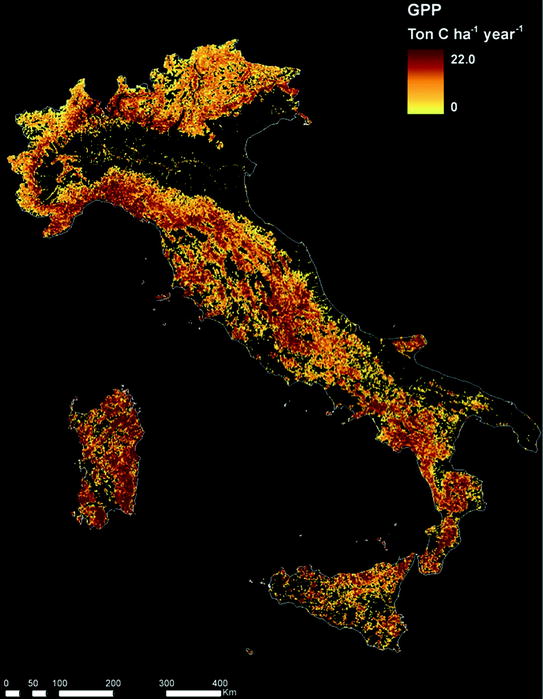
The NPP map of Italian forests simulated by the described modeling approach is shown in Fig. 5.1. The maximum NPP is around 900 g C m−2 year−1, and is prevalently found on the lowest Alpine and intermediate Apennines zones. As regards the forest types, the highest productions are obtained for species distributed over hilly-low mountain areas (i.e. deciduous oaks and chestnut), which are less affected by thermal and water limitations.
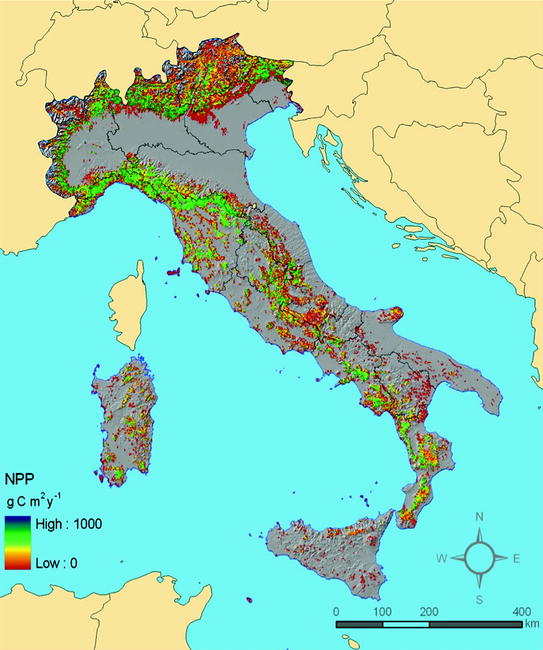
Fig. 5.1
Map of estimated NPP for Italian forests
Measured (INFC) and estimated forest CAIs are shown in the scatter plot of Fig. 5.2. A moderate accordance is observable (r = 0.617; RMSE = 2.04 m3 ha−1) and there is a tendency to underestimation (%MBE = −19.5). Most of this underestimation derives from Eq. 5.2, where FC A and NV A are computed using standing volumes which are significantly lower than those of INFC (%MBE = −23.6). It can therefore be concluded that the applied modeling strategy is capable of providing realistic regional CAI estimates using information completely independent of INFC measurements.
Fig. 5.2
Measured versus estimated forest CAI for all forest types and regions considered (n = 69; ** = highly significant correlation, P < 0.01)
5.2.2 Estimation of Italian Forest NPP. the 3-PG Model
Within the CarboItaly project, the NPP of the Italian forests has also been estimated through the application of a modified version of the widely used 3-PG model by Landsberg and Waring (1997). The 3-PG model as proposed by Nolè et al. (2013) is based on the 3-PGS (Spatial) model (Coops et al. 1998, 2005, 2007; Coops and Waring 2001; Nolè et al. 2009; Tickle et al. 2001) modified to run on a daily time step and produce estimates of GPP and NPP improving model reliability and maintaining the original simplified modeling approach at the same time.
The model fundamental assumption is the canopy LUE (light use efficiency) approach, considering the GPP as the product of the absorbed photosynthetically active radiation (aPAR) and ε max, which is assumed to be a biome-specific constant for potential LUE (g C m−2 MJ−1), and reduced by the effect of environmental constraints (f (x)). Daily GPP (g C m−2 MJ−1) has then been computed as follows:
(5.4)