Shipping Market Cycles
Chapter 9
Shipping Market Cycles
Martin Stopford*
1. Introduction
Shipping cycles create endless problems for shipping investors and analysts alike. The shipping industry, like Sisyphus, the mythological character condemned to pushing a stone up a hill, only for it to roll down again, seems to be caught in an endless sequence of cycles over which it has no real control. So why bother to issue warnings?1 How would Sisyphus have felt if each time he was half way up the hill some smart economist was standing there to warn him that the stone would soon be on its way down again? Shipowners feel the same way about the killjoy analysts intent on spoiling their bit of fun during the all-too-brief freight booms.
It is not just modern shipping executives who feel this sense of frustration. A century ago in his 1894 annual report, a London shipbroker spoke for all of us when he wrote:
“The philanthropy of this great body of traders, the shipowners, is evidently inexhaustible, for after five years of unprofitable work, their energy is as unflagging as ever, and the amount of tonnage under construction and on order guarantees a long continuance of present low freight rates, and an effectual check against increased cost of overseas carriage.”2
This masterpiece of understatement precisely captures the sense of dedication, purpose and deja vu that characterises shipping cycles today, as it obviously did a century ago. It also leaves shipping economists with a legitimate question about what they can really contribute to the commercial shipping industry as it beats its way through these cycles. Warnings aside, what have we to say?
In this chapter we study these cycles, or waves, in the shipping market. There are three main aims. First to look at some of the general characteristics of shipping cycles and discuss how they fit into the economics of the shipping market. Secondly we will study the historical pattern of cycles (if we decide they are cycles), so that we get an idea of the many different economic forces which contribute to their progress. We might call this “cyclical recognition”. Thirdly we will discuss the causes of cycles and focus more closely on the economic mechanisms which control them.
2. The Role of Cycles in Shipping Economics
Market cycles are the driving force behind shipping investment and chartering. They are the heartbeat of the shipping market, pumping cash in and out of the business. By forcing companies to compete with each other for a share of this wealth, the market lures them in the direction needed to give the most efficient use of resources. In fact the “cycles” are so much a part of the culture of the industry, that it seems hardly necessary to define them. However it is worth spending a little time discussing what the industry generally means by a cycle, and what impact the cycles have. This will help to give some perspective.
2.1 The characteristics of shipping cycles
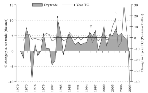
Strictly speaking a cycle is “an interval of time during which one sequence of a regularly recurring sequence of events is completed”.3 The cycle in Figure 1 is defined by its amplitude (A), which is the distance from peak to trough, and its frequency (F), which is the distance between peaks (or troughs) in the cycle. Viewed in this way a shape of a regular cycle C can be defined in terms of the values of A and F.

Of course nobody expects shipping cycles to be this regular. There is a widely held “rule of thumb” that they last seven years, but even a cursory examination of the tanker and bulk carrier market cycles in Figure 2 confirms that in the real world the periods of feast and famine bear little relationship to the stylised cycles in Figure 1.
The fact that the cycles are not regular makes it even more important to understand them, at least from the viewpoint of the shipping analyst. The practical importance of cycles cannot be understated. In July 2008 a 280,000 dwt tanker was earning $170,000 a day, but just 12 months later in 2009 it was earning only $11,000 a day. This volatility in earnings has a tremendous impact on the way everyone involved in the commercial operation of shipping views the business. For shipowners it offers an incentive to “play the cycle”, earning premium revenue when the market is high and, in an ideal world, fixing the ships on time charter or selling out just before the market moves in to a trough.

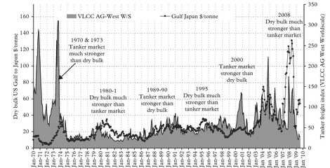
Source: Fearnleys, Clarkson Research Services Ltd
Another feature of the shipping cycle, illustrated by Figure 2, is the correlation between cycles in different segments of the market. The spot market rates in the tanker and bulk carrier markets are compared over the 39-year period 1970–2009. The timing of cycles in the two markets is broadly similar, but the correlation is far from perfect and in some cases the two market segments behave quite differently. In 1971 and 1973 the tanker market surged way ahead of the dry bulk market in a super-boom which the bulkers were not really included in. Note that the market remained firm through 1974 for almost a year after the 1973 oil crisis which happened in October 1973. But in 1980 the bulk carrier peak was longer and stronger than the rather feeble tanker upswing. Then in the late 1980s both markets moved up to a new peak, but this time the tanker market was much stronger than dry bulk. Bulkers peaked in 1995 when tankers had a tough year, but in 1997 the tanker market enjoyed a peak, during a rather bleak year for the bulk carrier market. But then it was the bulk carrier market’s turn, with a spectacular boom in 2007–2008 which the tanker market could not match. If nothing else this demonstrates that we cannot generalise about cycles by assuming that even closely related markets have the same peaks and troughs. On the contrary it suggests that different shipping segments are, to some extent at least, isolated from each other.
Even more prominent is the opportunity for “asset play”, a term often used to describe speculating on the sale and purchase of ships. Every shipping investor’s ambition is to buy in at the bottom of the cycle and sell at the peak. Historically this has always been an important part of shipowners’ revenues, especially during periods of inflation. The 1980s provided one of the most spectacular opportunities ever. A VLCC could be purchased in the mid-1980s for about $3 million, but by 1989 its price had gone up to almost $30 million, a tenfold increase in just five years. A Capesize bulk carrier bought for $25 million in 2002 could have been sold for $160 million in 2008. Of course the fact that the cycles are so irregular makes this a tricky game to play, but with so much at stake financially, who would expect it to be simple?
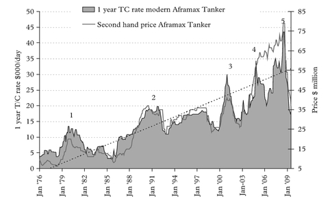
Source: author
Figure 3 illustrates the link between cycles is earnings and asset values by comparing the one-year Time Charter rate for a five-year-old Aframax Tanker (left axis) with its market value (right axis). The correlation coefficient of 0.87 is very close, with peaks and troughs following the same cyclical pattern, confirming the common sense expectation that the asset’s price will be correlated with its earning capacity. With such high volatility it is no wonder that shipowners spend so much time considering how to take advantage of this volatility by buying low and selling high.
In fact the causal mechanism underlying the cycles is simple enough. They are generated by changes in the delicate balance of supply and demand for ships. When demand increases faster than supply, freight rates and second-hand prices move up. Conversely when supply exceeds demand, freight rates are driven down by competition, and in many cases fall to the operating cost of the ship. But like many “simple” economic mechanisms, in practice it can develop in a host of different ways. In the next section of this chapter we will study the way cycles have behaved over 120 years of modern shipping. This provides some practical insights into the many different permutations of factors which can drive the supply and demand sides of the market. We will then look more closely at the cyclical mechanism and in particular the dynamics of the market cycle, in an effort to understand the economic framework itself.
3. A Brief History of Shipping Cycles, 1869–2002
A dry freight index covering the 140-year period from 1869–2009 is shown in Figure 4. Identifying the start and finish of each cycle is not always easy. Some cycles are clearly defined, but others leave room for doubt. Does a minor improvement in a single year,
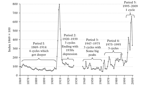
Source: Stopford (2009): Maritime Economics (Routledge), Annex C
as happened in 1877, 1894 or 1986, count as a cycle? There are several of these “minicycles” where the freight rates moved slightly above trend. However careful examination of the statistics and other information suggests that taking 1869 as the starting point4. I there were 15 dry cargo freight cycles during the 140-year period covered by the graph. For the purposes of discussion in this chapter we will divide this sequence of 15 cycles into five periods, which are marked in Figure 4. The first of these, period 1, covers one of the most exciting periods of modern shipping history, when much of the basic technology used by the industry today was developed. Period 2 covers a much more difficult phase between the World War I and the World War II, and of course it includes the Great Depression of the 1930s. Period 3 encompasses the second era of expansion between the end of the World War II and the first oil crisis in 1973. In a very different way this was another period when the shipping industry was adopting new technology in response to rapid trade growth. Period 4 covers the quarter-century from the first oil crisis through to the end of the twentieth century, including the second great shipping depression in the 1980s. Finally period 5 covers one of the most profitable periods in the shipping industry’s history, incorporating a single lengthy cycle which surged to a peak in 2008.
In the following sections we will review each of these periods, with two main aims. The first is to establish the general economic conditions which existed on the supply and demand sides of the shipping market during each period, to give us an idea of the overall tone of the market. Secondly we will look at the course the cycles took and try to get some sense of how the industry saw them at the time. In this way we can identify the turning points, marking the beginning and end of each cycle and the length of each trough. Finally we will examine the impact the cycles have had on shipping over the last century. Statistics give no sense of the real events underlying these cycles. For example the brief dips in the index during the 1930s and 1980s give no sense of the desperation and financial hardship which shipowners suffered during these periods. So if we are to obtain a better insight into the nature cycles, and their causes, we must focus more closely at what was going on in each period.
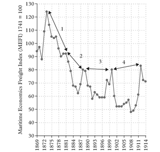
3.1 Period 1: Shipping cycles 1869–1914
The 45 years before 1914 provides an example of the tight interplay between short-term cycles and long-term supply/demand fundamentals. The freight index in Figure 5 shows a long-term downward trend from 100 in 1869 to 45 in 1908. To put this into cash terms, we can take the example of the freight rate for coal from South Wales to Singapore. In 1869 the freight was 27 shillings/ton, but by 1908 it had fallen to a low of 10 shillings5. Onto this long term trend was superimposed the series of four shorter cycles of about ten years in length.
This was a period of great activity on both the demand and supply sides of the shipping market. Driven by industrialisation and the expansion of the European empires, trade grew rapidly. Continuous advances in technology on the supply side of the shipping market helped the whole process, not least by reducing transport costs. Ships were becoming bigger and more efficient. In 1871 the largest transatlantic liner was the Oceanic, a 3,800 gt vessel with a 3,000 horsepower engine capable of 14.75 knots. It completed the transatlantic voyage in 9½ days. By 1913 the largest vessel was the 47,000 gt Aquatania. Its 60,000 horsepower engines drove it at 23 knots. The transatlantic voyage time had fallen to under five days. These vessels were
Source: Stopford (2009): Maritime Economics (Routledge), Annex C
comparable in length with a 280,000 dwt tanker and vastly more complex in terms of mechanical and outfitting structure.
Perhaps the most important technical improvement was in the efficiency of steam engines. With the introduction of the triple expansion system and higher pressure boilers the cargo payload of steamships increased rapidly. The early steam engines had worked at 6lbs/in pressure and consumed 10lbs of coal/horsepower per hour. They could carry little but bunker coal. By 1914, pressures had increased to 165lbs/in and coal consumption had fallen to 1½lbs/horsepower per hour, giving the steamer a decisive economic advantage, despite its high capital costs. The economic advantage of steam ships was compounded by economies of scale. As a result, the world fleet doubled from 16.7 million grt in 1870 to 34.6 million grt in 1910 and the continuous running battle between the new and old technologies dominated market economics as each generation of more efficient steamers pushed out the previous generation of obsolete vessels. The first to come under pressure were the sailing ships, which were replaced by steamers. In 1870 steamers accounted for only 15% of the tonnage but by 1910 they accounted for 75% of the world merchant fleet6. The growth in demand was matched by equally rapid growth in supply. As shipyards gained confidence in steel shipbuilding, production grew rapidly. Between 1868 and 1912 the shipbuilding output of the shipyards on the Wear, trebled from 100,000 grt to 320,000 grt. Change is never easy and the market used a series of cycles to alternately draw in new ships and drive out old ones. The cycles can be clearly seen in Figure 4 which shows peaks in 1871, 1881, 1889 and 1900.
Cycle 1 started in 1871, and lasted 10 years until 1881. During this period rates fell steadily, as a new generation of steamers competed with the sailing ships which continued to offer low-cost freight carriage. There was a slight recovery of rates in the second half of 1873, the year when Mr Plimsoll published “Our Seamen”, and started his campaign which led to the introduction of the Plimsoll line on ships. From there it was downhill all the way, with rates hitting a trough in 1879, driven by the “excessive and ever increasing supply of tonnage”. However in 1880 the market started to pick up and 1881, the peak of a business cycle in the United Kingdom, saw “in almost every trade a fair amount of business”. This good start lead to a second excellent year in 1882, described by brokers as being “exceedingly satisfactory”. A sure sign that a great deal of money was made.
Cycle 2 started almost immediately and rates fell through 1883 to a new trough in 1884. Brokers reported that rates were unprofitable for steamers, and even in the better months insufficient to provide for depreciation. The next three years from 1885 through to 1887 were still dull and highly competitive, with relatively low rates. By this time the newly founded liner business was working hard to establish conferences that would protect them. However things improved in 1887 and by 1888 brokers were reporting the year as “a remarkable one in the history of shipping. A transformation of the whole trade from abject depression to revival and prosperity”. Again we find that this coincided with a peak in the world trade cycle. The good times continued through 1889.
Cycle 3 commenced in earnest in 1890 when freight rates slumped, driven down by heavy deliveries which greatly exceeded the previous peak in the early 1880s. By 1892 the market was in severe depression and rates remained very depressed through 1894, and 1895. By 1896 the balance seems to have been partly restored and brokers report fluctuating rates which gave way to a much firmer market in 1898. This upward trend continued and the market moved to a peak in 1900 which was reported to be a memorable one for the shipping industry. Brokers reported “vast trade done and large profits safely housed”. This concluded the third cycle, which had lasted the greater part of the decade and was the worst so far.
Cycle 4 turned out to be another long recession. In 1901 the market crashed, leading to a series of very depressed years. This did not let up until 1909 when the market started to believe that the worst was over. For once they were right and 1910 was an excellent year. Once again the explanation of the long recession, at least as reported by the contemporary brokers, was a recession in trade which followed the great boom of 1900 and over production of ships.
So what was driving these “short” cycles? On the demand side, rapidly growing trade was dominated by the world business cycle, whose cyclical peaks in 1872, 1883, 1892 and 1903 roughly correspond to the peaks in the shipping cycles7. On the supply side shipbuilding production amplified the demand instability by overshooting during the booms. This combination laid the foundations for a sequence of cycles which got steadily longer, with the last one stretching out for the best part of a decade.