Chapter 31

Revisiting the Productivity and Efficiency of Ports and Terminals: Methods and Applications

Kevin Cullinane*

1. Introduction

Over the past decade, there has been a proliferation of research which investigates the efficiency of ports and terminals. Given the increasing prominence of container shipping within the maritime sector and the relative ease of analysis in situations where unit cargoes are standardised, it is not surprising that the majority of this work has been applied to the container port sector. It is also justified by the fact that container ports form a vital link in the supply chains of trading companies and nations worldwide. In terms of the logistics cost which they account for within any given supply chain, the level of a container port’s performance and/or relative efficiency will, to a large extent, determine the competitiveness of a nation and can ultimately have an influence upon industrial location decisions and the benefits derived from the economic policies of national governments. Thus, although productivity and/or efficiency analyses can provide a powerful management tool for port operators, they can also constitute a most important input to studies aimed at informing regional and national port planning and operation.

It is unfortunate, therefore that, in everyday use, the terms “productivity” and “efficiency” are used interchangeably. As a result, the precise meanings of the two terms have become blurred and indistinct. In the ensuing discussion of port and terminal productivity and efficiency, however, it is important to distinguish between them.

Productivity can very simply be defined as the ratio of outputs over inputs. This yields an absolute measure of performance that may be applied to all factors of production (inputs) simultaneously (as well as to all outputs) or to merely an individual factor of production. In this latter case, the outcome of such a calculation is more correctly referred to as a partial productivity measure. As is shown in the review contained in section 2 of this chapter, most historic analyses of port performance involved the calculation of partial productivity measures across a range of ports and/or terminals and the comparison of such calculated measures. Since the publication of the first edition of this handbook,¹ however, there has been a veritable explosion in the number of applications utilising the two main contemporary methods for the measurement of technical or productive efficiency. These more rigorous, holistic and scientific methodologies are introduced and described in detail in sections 4, 5 and 6 of this Chapter. Sections 5 and 6 also contain reviews of the major applications of each of these methods to the derivation of technical efficiency measures in the container port and/or terminal sector. Prior to that, in section 3 of this chapter, the theory underpinning the study of economic efficiency is presented.

2. Lessons Learned from Traditional Port Performance and Productivity Studies

The measurement of port efficiency is complicated by the large variety of factors that influence port performance.² The most obvious influences can be generalised as the economic input factor endowments of land, labour and capital. Dowd and Leschine³ argue, in fact, that port and/or terminal productivity measurement is a means of quantifying efficiency in the utilisation of these three resources. However, there are other influences that are not so easily classified, nor indeed even capable of being quantified, for the purpose of empirical investigation. A few examples of these influences include: the level of technology that is utilised in the operations of a port or terminal; the industrial relations environment within the port or terminal (and, hence, the risk of disruptions to the supply of labour); the extent of co-operation or integration with shipping lines and, as analysed in Cullinane and Song,⁴ the nature of the ownership of the port and the impact that this may have on the way that the port is managed and/or operated.

Despite these difficulties, attempts at estimating port or terminal productivity have been legion. This is particularly the case in container handling where, as might be imputed from the plethora of studies that focus on this sector, the need for high productivity or high efficiency levels is probably greater than in port facilities that concentrate on serving other forms of shipping.

Traditionally, the performance of ports has been variously evaluated by calculating cargo-handling productivity at berth (e.g.^5–7), by measuring a single factor productivity (e.g. labour as in the case of^8–10) or by comparing actual with optimum throughput for a specific period of time (e.g.¹¹).

Dowd and Leschine¹² approached the issue specifically in relation to container terminal productivity and highlight the fact that, probably because of the standard nature of the cargo that is handled in such facilities, there is an incessant demand in the industry for some form of universal standards or benchmarks for container terminal productivity. For the better terminals, there are obvious marketing advantages to be had from this. One major stumbling block in seeking to achieve such a standard is the lack of uniformity in productivity measurement across the sector. By way of exemplifying this, while some terminals will count rehandles and hatchcover removals as “moves”, others do not.

A second problem exists in that each participating player has a different interest in port or terminal productivity. For the port or terminal itself, the main goal may be to reduce the cost per unit of cargo handled and, thereby, raise profitability. For the port authority, the main goal may be to maximise the throughput per unit area of land that it leases to the terminal operator, so as to maximise the benefits derived from the investments it makes. For the carrier, the goal may be to minimise the time that a ship spends in port.

In an effort to provide a more rigorous and holistic evaluation of port performance, several alternative methods have been suggested, such as the estimation of a port cost function,¹³ the estimation of a total factor productivity index of a port¹⁴ and the establishment of a port performance and efficiency model using multiple regression analysis.¹⁵

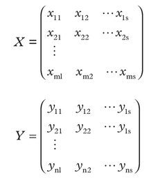
Chang ¹⁶ appears to have made one of the earliest efforts to estimate a production function and the productivities of inputs within the port sector. This was done for the port of Mobile in the US. In attempting to derive a port production function, the author focuses on general cargo-handling volume as a measurement of port performance and assumes that port operations follow the conventional Cobb-Douglas case as expressed by:

where

Y = annual gross earnings (in real terms)

K = the real value of net assets in the port

L = the number of labourers per year and the average number of employees per month each year

e^γ(T/L) a proxy for technological improvement in which (T/L) shows the tonnage per unit of labour.

The author argues that, for the estimation of a production function of this form, the output of a port should be measured in terms of either total tonnage handled at the port or its gross earnings.

De Neufville and Tsunokawa¹⁷ undertook an analysis of the five major container ports on the east coast of the US and derived an estimate of a container port production possibility frontier on the basis of the panel data collected. They deduced that Hampton Roads and Baltimore were consistently operating inefficiently during the period 1970–1978 and attributed this to poor management as the root cause. The findings highlight the importance of economies of scale in port/terminal productivity and, as such, the authors conclude that, because of the economic returns to be reaped, policy makers should promote and place greater investment into large load centre ports, rather than into the proliferation of smaller, more regionally focussed port developments.

Suykens¹⁸ points out that the measurement of productivity and subsequent comparison between ports is extremely difficult. Quite often, this is due simply to differences in the geophysical characteristics of the ports to be compared. For instance, there will be fundamental constraints on the productivity of ports where locks are needed, or which are located up river estuaries or in the middle of a port town as opposed to at a greenfield location. Difficulties also arise where the type of cargo handled at the comparison ports differ or when one port is primarily serving its own hinterland and another is primarily a transhipment port. Under all these scenarios, it would be fundamentally unfair and possibly misleading to make productivity comparisons on a straightforward basis. It may be argued, therefore, that in order to properly evaluate the performance of a port, it is important and necessary to place it within a proper perspective by drawing comparisons with other ports that operate in a similar environment.

Tongzon and Ganesalingam¹⁹ applied cluster analysis to compare the port performance and efficiency of ASEAN ports with counterparts overseas. The rationale for this analysis lay primarily with a purported requirement for such a comparison to be conducted only amongst ports that are similar in terms of their management or operational environment. The results suggested that the ASEAN ports, especially Singapore, were more technically efficient in terms of the utilisation of cranes, berths and storage areas, but that they were generally less efficient in terms of timeliness, labour and tug utilisation. In addition, it was deduced that port charges in ASEAN ports were significantly higher than those of their overseas counterparts falling within the same cluster (i.e. comparable ports).

Tongzon²⁰ elaborated upon this benchmarking concept by utilising an approach based on principal components analysis for the identification of suitable benchmark ports. Ashar²¹ is critical of this approach. In particular, the need for such an analysis to be conducted at the level of the terminal is highlighted by reference to the fact that several of the ports included in Tongzon’s sample were, in fact, landlord ports (as defined in²²).

Sanchez et al.²³ also apply principal components analysis to generate different port efficiency measures based on data from a survey of Latin American common user ports. These efficiency estimates are then incorporated as one of the explanatory variables in the estimation of a model of waterborne transport costs. Their analysis reveals that port efficiency, liner shipping calls, distance and value of goods are all significant determinants of waterborne transport costs and, therefore, impact directly on a nation’s competitiveness.

Braeutigam, Daughety and Turnquist²⁴ note that ports come in different sizes and face a variety of traffic mix. As such, they suggest, the use of cross-sectional time-series, or even panel data, may fail to show basic differences between ports; thus leading to a misjudgement as to each port’s performance. They attest, therefore, that it is crucial to estimate econometrically the structure of production in ports at the level of the single port or terminal, using appropriate data such as the panel data for a terminal. This view and suggested alternative approach also receives support elsewhere.^25–27

In undertaking the comparison of port productivities conducted within their study, Tongzon and Ganesalingham²⁸ compare ports on the basis of a basket of standard port productivity measures such as: shipcalls per port employee, net crane rate, ship rate, TEUs per crane, shipcalls per tug, TEUs per metre of berth, berth occupancy rate, TEUs per hectare of terminal area, port charges, pre-berthing time, berthing time and truck/rail turnaround time. Since the primary role of ports is to facilitate the movement of cargoes, the authors recognise that it is vital to evaluate port performance in relation to how efficient are their services from the perspective of the port user: the shipowners, shippers (importers and exporters) and the land transport owners. It is obvious, therefore, that port performance assessment cannot be based on a single measure. As is clear from the list of productivity measures employed, whilst it does contain certain operational productivity measures, it also recognises that this is only meaningful to port users when it translates into lower costs to them.

Frankel²⁹ is highly critical of the productivity measures that are applied in ports when he suggests that most port performance standards are narrowly defined operational measures that are useful only for comparison with ports that have similar operations or against proposed supplier standards. He asserts that port user interest in port productivity (and the service quality that it relates to) is much more wide-ranging and it is vitally important that ports attempt to address this disparity in outlook. Port users, he asserts, are concerned with issues such as the total time and cost of ship turnarounds and (increasingly) of cargo throughput. The realignment of what a port considers to be valid performance measures is required because the commercial environment of port operations is becoming increasingly competitive as hinterlands overlap. In such a context, port users have a real choice in the selection of the ports that they want to use.

The focus which Frankel advocates, on the port users’ perspective of port efficiency, is particularly interesting and important in that it shifts the need for, and usefulness of, valid port and/or terminal productivity and efficiency measures away from the fulfillment of an internally-oriented managerial (cost minimisation) objective and towards an externally-oriented marketing (revenue-maximisation) objective.

Chapon³⁰ specifically states that the overall cost of cargo-handling in a port comprises two separate components: the cost price of the actual handling and the cost price of immobilizing the seagoing vessel for the period of its stay in port. In other words, this second cost is, in economic terms, the opportunity cost associated with the revenue lost or, in the terminology of logistics, the cost of lost sales. This second component has risen to even greater prominence as ships have become increasingly expensive (i.e. exhibiting high fixed to variable cost ratios), a feature that is particularly relevant to the liner trades over recent years. Several studies of productivity have adopted this perspective in undertaking productivity measurement and comparisons.^{31, 32} It is fundamentally this perspective which has prompted the plethora of OR-based analyses of ship–shore interactions aimed at optimal crane deployment and/or loading/unloading operations, a comprehensive review of which is provided by Stahlbock and Voss.³³

All this points to the fact that productivity levels in ports have implications for the real cost of loading and discharging a ship. Suykens,³⁴ however, points to the need for caution in making such comparisons since the higher productivity in a port may be reflected in the wages it pays and/or the depreciation charges it incurs as the result of the investment in state-of-the-art equipment that has been made. Both of these influences on higher port productivity will be mirrored in the port tariff that is charged. Thus, there is a need for a balanced and joint view of both port pricing and productivity. Other commentators have pointed to the need to assess the range of prices payable for different levels of port productivity within the context of the effectiveness of service provision.³⁵ This, of course, has prompted empirical studies of the quality of port performance as an adjunct to the many analyses, using very varied methodologies, which focus on the quantitative assessment of relative port productivities.³⁶

Ports have an interaction with other parts of the logistical chain. Indeed, the suggestion has been made that the real value of productivity improvements in ports depends upon whether this results in an improvement to the efficiency of the total logistical system or whether it merely shifts a “bottleneck” from one part of the system to another.³⁷ This calls for the adoption of a still wider perspective on the issue of port productivity and efficiency.³⁸

In relation to the issue of technical efficiency rather than productivity measurement and comparison, it can be deduced that by the very nature of investments in cargo handling technology and the expansion of space in ports, additions to capacity have to be large compared to the existing facilities. In other words, when investments are made, they are made primarily on an ad hoc basis and with a view to future expectations of expanded demand. In consequence, since available capacity cannot be fully utilised in the years immediately following the time that such investments in additional capacity come on stream, then technical inefficiency is inevitable.

In any analysis of a single port’s time series of technical efficiency, therefore, the situation must be defined by numerous inefficient observations being bounded by a comparatively few observations that are deemed efficient. Because of this characteristic (i.e. that efficiency in operations cannot be assumed), De Neufville and Tsunokawa³⁹ point to the inadequacy of any approach that is based on a least squares regression analysis to estimate the production function for the industry. This is because any such analysis has to be based on the complementary assumptions that all observations are efficient but that any deviation of an observation from the production function is due to random effects. Without explicitly acknowledging the fact, this assertion points to the need for the adoption of contemporary approaches to the measurement of efficiency.

3. The Economic Concept of Efficiency

In simple terms, the performance of an economic unit can be determined by calculating the ratio of its outputs to its inputs; with larger values of this ratio associated with better performance or higher productivity. Because performance is a concept that is only meaningful when judged relatively, there are many bases upon which it may be assessed. For instance, a car manufacturer uses materials, labour and capital (inputs) to produce cars (outputs). Its performance in 2010 could be measured relative to its 2009 performance or could be measured relative to the performance of another producer in 2009, or could be measured relative to the average performance of the car industry, and so on.

Economic efficiency relates specifically to a production possibility frontier; an economic concept which is useful in explaining two distinctive concepts of efficiency: productive (or technical) efficiency and allocative efficiency. In economic theory, costs can exceed their minimum feasible level for one of two reasons. One is that inputs are being used in the wrong proportions, given their prices and marginal productivity. This phenomenon is known as allocative inefficiency. The other reason is that there is a failure to produce the maximum amount of output from a set of given inputs. This is known as productive (or technical) inefficiency. Both sources of inefficiency can exist simultaneously or in isolation. As implied above, these sources of inefficiency can be easily explained by using the concept of a production frontier.

An economic unit operating within an industry is considered productively (technically) efficient if it operates on the frontier, whilst the unit is regarded as productively inefficient if it operates beneath the frontier. When information on prices is available and a behavioural assumption (such as profit maximisation or cost minimisation) is properly established, we can then consider allocative efficiency. This is present when a selected set of inputs (e.g. material, labour and capital) produce a given quantity of output at minimum cost, given the prevailing input prices. An economic unit is judged allocatively inefficient if inputs are being used in the wrong proportions, given their prices and marginal productivity.

Fundamentally, however, the technical efficiency of an entity is a comparative measure of how well it processes inputs to achieve its output(s), as compared to its maximum potential for doing so – as represented by its production possibility frontier, which is widely used to define the relationship between inputs and outputs by depicting graphically the maximum output obtainable from the given inputs consumed. In so doing, the production frontier reflects the current status of technology available to the industry. By implication, therefore, the production possibility frontier of an entity may change over time due to changes in the underlying technology deployed.

In the container port sector, an example might be the greater reach of contemporary gantry cranes over their historic counterparts. Over the past decade in particular, this innovation in technology has facilitated a very significant improvement in partial productivity measures such as container moves per hour. Depending upon the relationship between the cost of investing in such cranes and the reduction in operating cost per container moved, it could also mean greater output for the same level of input at all scales of production (i.e. this represents an outward move in the production possibility frontier). If it could be established that this innovation has led directly to an improvement in the overall (total factor) productivity of the port (even where this compares favourably to that of other suitable benchmark ports), but that the new cranes like the old ones were still being optimally employed at full capacity, then a situation would exist where technical efficiency has remained the same (i.e. at a maximum), but there has been an improvement in productivity (even comparatively).

In a similar fashion, the scale of output(s) or inputs can be altered to take advantage of efficiencies due to scale. This too may mean that an entity can remain at 100% technical efficiency (so that output is at the maximum possible level for a given level of input) by moving along the production possibility frontier, but that its (total factor) productivity can simultaneously increase. It may be inferred from this explanation that technical efficiency and productivity also have time-scale connotations, whereby the former is much more of a long-term phenomenon, while the latter is a concept that is grounded more firmly in the short-term (see Coelli, Prasada Rao and Battese⁴⁰ for a comprehensive treatment of productivity and the different forms of efficiency).

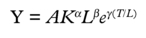
With respect to how to measure the different sources of (in)efficiency, let us suppose that the production frontier of an economic unit is as depicted in Figure 1 and can be denoted by Y = f (x₁, x₂ ), where two inputs (x₁ and x₂ ) are used, in some combination, to produce one output (Y). It is also assumed that the function is characterised by constant returns to scale. In this case, the isoquants Y_A and Y_B indicate all possible combinations of x₁ and x₂ that give rise to the same level of output.

Assume that the firm’s efficiency is observed at point A, rather than C. This position is neither allocatively nor productively efficient. Its level of productive efficiency is defined as the ratio of OB/OA. Therefore, productive inefficiency is defined as 1-(OB/OA) and can be interpreted as the proportion by which the cost of producing the level of output could be reduced given the assumption that the input ratio (x₁/x₂ ) is held constant. Under the assumption of constant returns to scale, productive inefficiency can also be interpreted as the proportion by which output could be increased by becoming 100% productively efficient. The level of allocative efficiency is measured as OD/OB (or C₁/C₂). Thus allocative inefficiency is defined as 1-(OD/OB) and measures the proportional increase in costs due to allocative inefficiency.

Consider position B in Figure 1. At this point, the firm is allocatively inefficient since it can maintain output at Y but reduce total costs by changing the input mix to that

Figure 1: A firm’s frontier production function

which exists at point C. At point B, however, the firm is productively efficient since it cannot increase output with this input combination of x₁ and x₂ and, given a suboptimal input mix (i.e. allocative inefficiency), the firm has minimised the cost of producing this level of output.

4. Introduction to More Contemporary Methods of Efficiency Measurement

In the last decade of the twentieth century, a family of methods for measuring efficiency were proposed which revolve around utilising the economic concept of an efficient frontier. Under this concept, efficient decision-making units (DMUs) are those that operate on either a (maximum) production frontier or a (minimum) cost frontier. In contrast, inefficient DMUs operate either below the frontier when considering the production frontier, or above it in the case of the cost frontier. Relative to a DMU located on a production frontier, an inefficient operator will produce less output for the same cost. Analogously, relative to any DMU located on a cost frontier, an inefficient operator will produce the same output but for greater cost.

As suggested by Bauer,⁴¹ there are several reasons why the use of frontier models is becoming increasingly widespread:

• the notion of a frontier is consistent with the underlying economic theory of optimising behaviour;
  
• deviations from a frontier have a natural interpretation as a measure of the relative efficiency with which economic units pursue their technical or behavioural objectives; and
  
• information about the structure of the frontier and about the relative efficiency of DMUs has many policy applications.

The literature on frontier models was inaugurated in the seminal contribution of Farrell,⁴² who provided a rigorous and comprehensive framework for analysing economic efficiency in terms of realised deviations from an idealised frontier isoquant. The proliferation of attempts to measure economic efficiency through the application of the frontier approach can be attributed to an interest in the structure of efficient production technology, an interest in the divergence between observed and ideal operation and also to an interest in the concept of economic efficiency itself.

Within the family of models and methods that are based on the frontier concept, a distinction exists between those methods that revolve around a parametric approach to deriving the specification of the frontier model and those that utilise non-parametric methods. Another distinction exists with respect to whether the model employed is stochastic or deterministic in nature. With the former, it is necessary to make assumptions about the stochastic properties of the data, while with the latter it is not. The nonparametric approach revolves around mathematical programming techniques that are generically referred to as Data Envelopment Analysis (DEA). The parametric approach, on the other hand, employs econometric techniques where efficiency is measured relative to a frontier production function that may be statistically estimated on the basis of an assumed distribution.

Econometric approaches have a strong policy orientation, especially in terms of assessing alternative industrial organisations and in evaluating the efficiency of government and other public agencies. Mathematical programming approaches, on the other hand, have a much greater managerial decision-making orientation.^43–45 Several studies^46–48 have compared the performance of alternative methods for measuring efficiency, focusing on the econometric method (in particular, the stochastic frontier model) and the mathematical programming method. As measured by the correlation coefficients and rank correlation coefficients between the true and estimated relative efficiencies, the results show that when the functional form of the econometric model is well specified, the stochastic frontier approach generally produces better estimates of efficiency than the approaches based on mathematical programming, especially when measuring DMU-specific efficiency where panel data are available. In addition, certain authors consider that the econometric approaches have a more solid grounding in economic theory.^49,50

5. Data Envelopment Analysis

5.1 Method

Data Envelopment Analysis (DEA) can be broadly defined as a non-parametric method for measuring the relative efficiency of a DMU. The method caters for multiple inputs to, and multiple outputs from, the DMU. It does this by constructing a single “virtual” output that is mapped onto a single “virtual” input, without reference to a pre-defined production function.

There has been a phenomenal expansion of the theory underpinning DEA, the methodology itself and applications of the methodology over the past few decades.^51–54 A significant stimulus to this corpus of literature came with the publication of a seminal

Figure 2: DMU and homogeneous units

work on the topic by Charnes, Cooper and Rhodes in 1978.⁵⁵ This work espoused a model for solving the DEA linear programming problem which has subsequently become widely known by the acronym of the authors’ surnames; the CCR model. The significance and influence of this paper is reflected in the fact that by 1999, it had been cited over 700 times in other papers incorporating applications of the DEA methodology or concerned with the theory or methodology of DEA. ⁵⁶

In common with other approaches based on the frontier approach, the fundamental idea in DEA is that the efficiency of an individual DMU⁵⁷ or Unit of Assessment⁵⁸ is compared relative to a bundle of homogeneous units. Implicit in this idea is the assumption that each individual DMU exercises some sort of corporate responsibility for controlling the process of production and making decisions at various levels of the organisation, including daily operation, short-term tactics and long-term strategy.

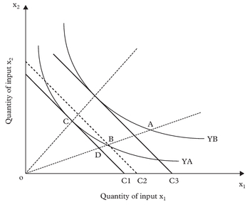
Figure 2 illustrates that DEA is used to measure the relative efficiency of a DMU by comparing it with other homogeneous units that transform the same group (types) of measurable positive inputs into the same group (types) of measurable positive outputs.

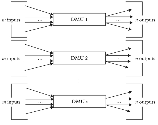
In the ports context, for example, DEA may be applied to compare the relative efficiency of a single container terminal to a set of other container terminals where the common output may be defined in terms of an annual throughput measured in TEU. Similarly, in this case, the common inputs may be the annual financial costs incurred in the provision of capital, land and labour or, alternatively, physical proxies for these factor inputs such as total length of berths, container stacking capacity, number of cranes, number of employees, total land available etc. The input and output data for Figure 2 can be expressed in terms of matrixes denoted by X and Y as shown below, where the element x_ij in the matrix X refers to the i^th input data item of DMU j, whereas the element y_ij represents the i^th output data item of DMU j. In X, there are m input variables and in Y, there are n output variables. In both input and output matrices, there are s DMUs considered.

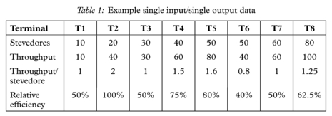
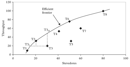
The basic approach to utilising DEA to measure the relative efficiencies of DMUs can be explained by the following example. Table 1 presents some basic production statistics for eight hypothetical container terminals. The “Throughput/stevedore” in Table 1 can be interpreted as a standard productivity measure. In an extremely simplistic sense that is useful for the purpose of illustrating the basic approach to DEA, this productivity measure can be employed to determine a simplistic and concise form of “relative efficiency” by comparing all DMUs against the best in the sample.

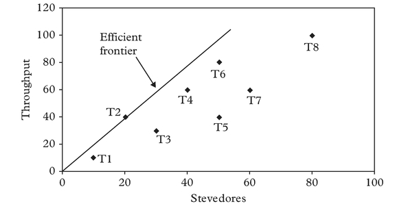
From Figure 3 it is clear that in terms of the particular relationship between inputs and outputs that we are looking at here (i.e. throughput/stevedore), T2 is the most efficient container terminal compared with the others (as represented by the other points on the graph). The straight line from the origin that passes through T2 can be termed an “efficient frontier” since all points along it have the maximum observed productivity measurement of one for throughput per stevedore. All the other points are inefficient compared with T2 and are “enveloped” by the efficient frontier. Within the context of DEA, the relative efficiencies of these other container terminals, as shown in the bottom line of Table 1, are measured by comparing the productivity measure (i.e. in this case throughput/stevedore) for each of these “inefficient” container terminals with that of T2. The term “Data Envelopment Analysis” stems from the fact that the efficient frontier “envelops” the inefficient observations and that they, in turn, are “enveloped” by the frontier.

Figure 3: Theoretical comparison of efficiencies of container terminals (CCR model)

It should be apparent that the complexity of measuring true relative efficiency (or indeed of even simply portraying the problem graphically) increases exponentially as the number of total input and output variables increase. It is this difficulty that the CCR model overcomes. This is because it was specifically devised to address the measurement of relative efficiencies of DMUs with multiple inputs and outputs.

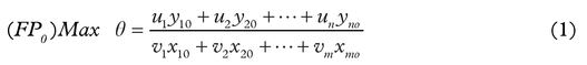
The CCR model can be expressed as the following fractional programming problem (1)–(4):

Subject to:

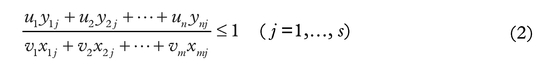
Given the data matrices X and Y shown earlier, the CCR model measures the maximum relative efficiency of each DMU by solving the fractional programming problem in (1) where the input weights v₁, v₂, … v_m and output weights u₁, u₂, … u_n are variables to be obtained. o in (1) varies from 1 to s in relation to the s optimisations that are required for all s DMUs. The constraint in (2) defines the fact that the ratio of “virtual output” (u₁ y₁₀ +u₂y₂₀ +…+u_n y_no ) to “virtual input” (v₁ x₁₀ +v₂ x₂₀ +…+v_m x_mo) cannot exceed unity for each DMU. This Fractional Programming (FP) problem represented in equations (1)–(4) has been proved to be equivalent to the following Linear Programming (LP) formulation shown in equations (5)–(9).⁵⁹

Subject to

It is important to recognise and note that the computation of the DEA CCR model has been greatly facilitated by the transformation from its original Fractional Programming (FP) formulation into a Linear Programming (LP) form of the model. This transformation has contributed greatly to the rapid development of the DEA technique and the proliferation of DEA applications. This has occurred because the solution of LP problems has a long-established history where numerous sophisticated computational methods have been developed and where commercial software packages are widely available. As such, calculating the complicated relative efficiencies of DMUs with multiple inputs and outputs is then rendered a comparatively simple task.

One assumption that underpins the early DEA approaches, including the CCR model, is that the sample under study exhibits constant returns to scale. There is a voluminous body of evidence that suggests that this assumption is particularly inappropriate to the ports sector where, it is quite commonly asserted, economies of scale are quite significant.^60–62 To cater for such situations where variable returns to scale may be more the norm, the CCR model has been modified so that scale efficiencies, for example, may be separated out from the pure productive (or technical) efficiency measure that the standard CCR model yields.

The main modified forms of the CCR model that are utilised in practice are referred to as the Additive model and the BCC model, the latter being named after its creators.⁶³ Accordingly, the efficient frontiers that are estimated by these models are different from that of the CCR model.

Figure 4 shows a hypothetical efficient frontier for situations when either the Additive or BCC models are applied to a sample of container terminals (i.e. there is an assumption that variable returns to scale prevail). In this illustrative example, the sample observations denoted by T₁, T₂, T₆ and T₈ lie on a non-linear efficient frontier and are all defined as efficient since each observation cannot dominate any of the others given the condition of variable returns to scale. The other points that are ‘enveloped’ by (i.e. lying below) these technically efficient points are deemed inefficient.

The Additive and BCC models are identical in terms of the efficient frontiers that they estimate. The main difference between them is the projection path to the efficient frontier that is employed as the basis for estimating the levels of relative (in)efficiency for those DMUs in the sample that are not located on the efficient frontier. For instance, in Figure 4, for the BCC estimate of inefficiency, the inefficient observation T3 can be projected either to T3_I or T3_O depending upon whether an input or output orientation is adopted. For the Additive model, however, T3 will be projected to T2 on the efficient frontier. This different approach to projection determines the different relative efficiencies for different inefficient DMUs. This is because the level of (in)

Figure 4: A comparison of container terminal efficiency (BCC and additive models)

efficiency for inefficient observations is derived from the distance it is located from the efficient frontier; a measure that is, of course, dependent upon the projection path that is utilised.

Irrespective of which model is selected for application, the main advantages of utilising a DEA approach to efficiency estimation can be summarised as follows:

1. both multiple outputs and multiple inputs can be analysed simultaneously;
   
2. more extraneous factors that have an impact on performance can be incorporated into the analysis (such as those relating to the commercial and competitive environment of the port operation, as well as other qualitative factors);
   
3. the possibility of different combinations of outputs and inputs being equally efficient is recognised and taken into account;
   
4. there is no necessity to pre-specify a functional form for the production function that links inputs to outputs, nor to give an a priori relationship (by pre-specifying the relative weights) between the different factors that the analysis accounts for;
   
5. rather than in comparison to some sample average or some exogenous standard, efficiency is measured relative to the highest level of performance within the sample under study; and
   
6. specific sub-groups of those DMUs identified as efficient can be ring-fenced as benchmark references for the non-efficient DMUs.

In the specific case of port efficiency, the ability to handle more than one output is a particularly appealing feature of the DEA technique, because a number of different measures of port output exist that may be used in such an analysis, with the selection depending upon what aspect of port operation constitutes the main focus of the evaluation. Surprisingly, however, this capability is rarely utilised in practice, with a clear preference amongst empirical analyses for focusing solely on a single output, most usually container throughput.

In addition to providing relative efficiency measures and rankings for the DMUs under study, DEA also provides results on the sources of input and output inefficiency, as well as identifying the benchmark DMUs that are utilised for the efficiency comparison. This ability to identify the sources of inefficiency could be useful to port and/or terminal managers in inefficient ports so that the problem areas might be addressed. For port authorities too, they may provide a guide to focusing efforts at improving port performance.

5.2 Applications

Applications of the DEA approach to efficiency estimation in the general transport industry are now quite common and examples exist of applications to virtually all modes. (This section is based on Cullinane and Wang, (see endnote 76) but has been supplemented by a review of more recent applications.) For example, a comprehensive review of DEA applications and other frontier-based approaches to the railway industry was conducted by Oum et al.⁶⁴ Similarly, De Borger et al.⁶⁵ carried out just such a review for attempts to measure public transit performance. It is with the air industry, however, that the greatest proliferation of DEA applications may be found.^66–72 This is interesting because of the great similarity that exists between the air and maritime industries, particularly the analogous positions of ports and airports; a feature that would suggest that there remains great scope for further applications of the DEA approach to the port sector.

In relation to the applications of DEA to ports that have already been undertaken, it is particularly interesting that there has been very little correspondence between the studies as to the choice of input and output variables that are considered. As Thanassoulis points out,⁷³ this is significant because the identification of the inputs and the outputs in the assessment of DMUs tends to be as difficult as it is crucial. In addition, Ashar et al.⁷⁴ attribute a lack of transparency to the use of the DEA technique as applied to the estimation of port and/or terminal efficiency.

Roll and Hayuth⁷⁵ were the first commentators to explicitly advocate the use of DEA for the estimation of efficiency in the port sector. By presenting a hypothetical application of the methodology to a fictional set of container terminal data, they reveal what potential the approach might hold. They point particularly to the applicability of the DEA approach to the measurement of productive efficiency in the service sector. In addition, they highlight the fact that while the DEA approach does not require a pre-specified standard against which to benchmark the performance measurements pertaining to an individual port or terminal, such standards can be incorporated into the analysis should this be desirable. This latter characteristic is particularly important in countering the argument that the weights estimated by DEA might be either misleading or, indeed, fundamentally wrong as a result of the possibility that they may be different from some prior knowledge or widely-accepted views on the relative values of the inputs or outputs.⁷⁷

Martinez-Budria et al.⁷⁸ use DEA to analyse the relative efficiency of the Spanish Port Authorities over the period 1993–1997. The methodology as they apply it involves the classification of the 26 different ports within their sample into three categories according to their “complexity”. This classification system would appear to be highly correlated to the size and/or throughput of the ports considered in the analysis. The results of the analysis reveal that the three groupings followed three distinct evolutionary paths in terms of relative efficiency. The most “complex” ports (i.e. roughly equating to those of largest size and throughput) display the highest levels of efficiency in absolute terms and a high growth rate in efficiency over time. Ports in the medium level of ‘complexity’ category displayed only low levels of efficiency growth over the sample period, while ports of low ‘complexity’ actually yielded a negative trend in relative efficiency levels during the period under study. This seems to suggest that not only are there significant economies of scale to be reaped in port operation, but also that this and other factors may be contributing to a concentration of cargo throughput in larger ports. It can also be inferred that the diminishing role of the smaller ports has an adverse impact upon their relative efficiency levels that, in turn, creates a vicious circle of cargo diversion away from this group of ports. By analysing the value of the slack variables to emerge from solving the DEA Linear Programming problem, this study found that the worst source of inefficiencies were, in general, due to excess capacities.

Tongzon⁷⁹ uses both DEA-CCR and DEA-additive models to analyse the efficiency of four Australian and 12 other international container ports for 1996. This cross-sectional efficiency analysis incorporates two output and six input variables, the data for which was collected for the year 1996. The output variables are cargo throughput and ship working rate, where the former is the total number of containers loaded and unloaded in TEUs and the latter is a measure of the number of containers moved per working hour. The input variables considered in the analysis were the number of cranes, number of container berths, number of tugs, terminal area, delay time (the difference between total berth time plus time waiting to berth and the time between the start and finish of ship working) and the number of port authority employees (as a proxy for the labour factor input).

Without precise a priori information or assumptions on the returns to scale of the port production function, two sets of results – for the CCR and Additive DEA models – are presented and discussed. A comparison of the results reveals that the CCR model identifies slightly more inefficient ports (six vs three) than the Additive model. As the author points out, this is not a surprising result as the CCR model assumes constant returns to scale, while the Additive model is based on the assumption of returns to scale that are variable. In consequence, the latter will require a larger number of ports to define the non-linear efficiency frontier.

The results of the initial analysis seemed to suggest that the model was over-specified for the sample size (i.e.