Representing Organizational Uncertainty

occurrences extracted from the whole corpus without replacement. The probability distribution for a sampling without replacement under the hypothesis of independence is the hypergeometric distribution (Ayuso et al. 2002), which contrasts with the binomial distribution (with replacement). Or in other words, the “probability of obtaining k items, of one out of two categories, in a sample of n items extracted without replacement from a population of N items that has 
$D = pN$
items of that category (and 
$(1-p)N = qN$
items from the other category)” (Marques de Sá 2007).


Results showed that the word guardia [on-call] turned out to be over-represented in the subcorpus JJ, the one from junior judges. Furthermore, this over-representation was found to be significant (Ayuso et al. 2003).

The data available in that survey, though, were limited. Questions were general, not specific, and answers were too short to allow any further text exploration. This led to our current survey on Spanish junior judges, which, on one hand, was specifically focused on junior judges, and on the other was designed to gather the types of problems that sprang from on-call situations.

Having rich textual data—part of it specifically focused on on-call problems—permits a variety of research strategies in order to both gather relevant data for modelling a knowledge base, and advance in our understanding of the problems faced by judges at courts when on-call.


5.2.1 Corpora


In order to carry out our analysis, we use three different textual corpora. These are composed by the set of responses to the open-ended questions contained in our survey. In particular, these questions were:


  • A question about the main types of problems regarding civil issues during the first appointment.


  • A question about the main types of problems regarding criminal issues during the first appointment.


  • A question about the main types of problems during on-call periods.

Since interviews were recorded, each answer was literally transcribed and saved in a different text file. Thus we have three different corpora (i.e., sets of responses) that contain a number of text files, each of which representing a single answer to a particular question. The three corpora are thus named and described:


  • civil: The collection of all responses regarding problems about civil issues, each document representing one single answer. It contains 111 responses out of 118 interviewed judges. Out of the 7 lacking respondents, 4 did not accept a recording, while 3 were not able to recall a single civil problem during the interview.


  • criminal: The collection of all responses regarding problems about criminal issues, each document representing one single answer. It contains 109 responses out of 118 possible responses. Out of the 9 lacking responses, 4 were due to non recorded interview, while 5 respondents were not able to recall any problem specifically related to criminal issues.


  • on-call: The collection of all responses regarding problems about on-call issues, each document representing one single answer. It contains 110 responses out of 118. As already noted, half of them were not recorded, while the other half were not able to recall any on-call problem at that moment.

Finally, Table 5.1 summarizes the state of each corpus regarding respondents and non-respondents.


Table 5.1
Number of respondents and non respondents for each corpus


Corpus

Responses

Expected

No record

No answer

Actual

Civil

118

4

3

111

Criminal

118

4

5

109

On-call

118

4

4

110

Total

354

12

12

330


5.2.2 Text as Data


Our hypotheses involve, on one hand, testing whether our textual corpora (civil, criminal, and on-call problems) are significantly different from each other, and on the other exploring the content of these corpora in a systematic way. Note that in both cases we treat text as data. We assume that the significant differences among documents can be reduced to differences in the use of language in the documents. Specifically, if two documents refer to different topics (e.g. they refer to different kinds of problems), these differences can appear in both the types of words they contain, and the frequency of these words. We apply statistical methods to these textual data in order to account for these differences in meaningful ways.

Using text as data to extract relevant social or political information in systematic ways is an old practice in political science (e.g. Lasswell et al. 1949). Compared to classical content analysis, computer-assisted text analysis (CATA) has peaked recently due to the ease of access to massive amounts of textual data (Grimmer and Stewart 2013), with applications in the analysis of party manifestos (e.g. Klingemann et al. 2006), media political content (e.g., Sementko and Valkenburg 2000), actor influence in policy dynamics (Klüver 2009), or the analyisis of coalition dynamics (Falcó-Gimeno and Vallbé 2013).

A number of reasons support the use of computerized methods for textual data analysis over semi-automated or even manual methods. On one hand, CATA-based research strategies are less time- and resource consuming than classical content analysis, the latter being highly dependent upon human or semi-automatic codification of units of text (Budge et al. 2001; Klingemann et al. 2006; Jones and Baumgartner 2012), which in times of large amounts of available textual information turns out to be a serious shortcoming. On the other hand, CATA techniques are better equipped to deal with potential measurement problems that typically affect classical content analysis projects (Neuendorf 2002; Krippendorff 2004; Benoit and Laver 2007; Budge and Pennings 2007a, b; Benoit et al. 2009).

Text may be analysed automatically at different levels responding to the research purpose at hand. Lower units such as words, sentences or text chunks are often used to account for the identification of semantic features within relatively extensive corpora, while whole documents (be they simple queries, court decisions or party manifestos) are usually taken for classification and scaling. In particular, Natural Language Processing (NLP), Machine Learning, and Text Mining techniques (e.g., multiple correspondence analysis, principal components analysis, multidimensional scaling and hierarchical clustering) have been widely used for topic identification (Lebart and Salem 1988), semantic extraction (Reinert 2000; Schonhardt-Bailey 2005, 2008), semi-automated dictionary construction (Young and Soroka 2012), and document scaling and classification (Srivastava and Sahami 2009; Falcó-Gimeno and Vallbé 2013).


Table 5.2
Descriptive statistics of the textual corpora used in the analysis


Corpora

N docs

Min.

Mean

Median

Max.

Std. Dev.

Tokens

Types

On call

110

21

664.1

459

3692

742.7

73,048

3290

Civil

111

5

380.5

115

5027

782.4

36,147

2685

Criminal

109

11

454.8

192.5

3339

634.3

42,748

2925

Regardless of the method applied, though, we must begin with a basic description of our textual data. To this effect, Table 5.2 presents basic descriptive statistics based on the word frequency of each document of the three corpora. We observe, first, that the On-call corpus is by far the larger of the three, with just above 73,000 word occurrences (tokens) and 3290 different words (types). Accordingly, the documents within the On-call corpus present a higher average frequency. Nevertheless, the three corpora have some similarities. First, all three present large differences regarding the word count of their documents. Note that in three cases there are documents with a very low word count (e.g., there is a document with just five words in the Civil corpus), and documents with a very large number of words (the larger document in the Civil corpus has 5027 words). The fourth and fifth columns of the table present measures of concentration. The fact that the median number of words is larger than the mean indicates a larger number of low-frequency documents in all three corpora. The standard deviation indicates the average distance between document frequencies and the mean frequency.

In order to compare the content of the documents through statistical methods to textual data we adopt the Bag of Words (or Vector Space) Model, that represents documents as vectors in a common vector space and is widely used in text mining and information retrieval (Salton et al. 1975; Baeza-Yates and Ribeiro-Neto 1999; Manning and Schütze 1999; Jakulin and Buntine 2004; Manning et al. 2008; Fortuna et al. 2009). Consider a corpus D that contains a number n of documents d:


$$\begin{aligned} D=\{d_1,d_2,d_3,{\ldots},d_n\}\end{aligned}$$

In turn, each document d has a number m of terms t:


$$\begin{aligned} d=\{t_1,t_2,t_3{\ldots},t_m\}\end{aligned}$$

Each term t occurs with frequency 
$tf_{t,d}> 0$
” src=”/wp-content/uploads/2015/10/A309690_1_En_5_Chapter_IEq4.gif”></SPAN>, which denotes the frequency of term <SPAN class=EmphasisTypeItalic>t</SPAN> in document <SPAN class=EmphasisTypeItalic>d</SPAN>. The frequency of all <SPAN class=EmphasisTypeItalic>m</SPAN> terms in a document <SPAN class=EmphasisTypeItalic>d</SPAN> will then be:</DIV><br />
<DIV class=Para><br />
<DIV id=Equc class=Equation><br />
<DIV class=EquationContent><br />
<DIV class=MediaObject><IMG alt=

This way, each document d can then be represented as a a “bag of words” with repeated elements (each one repeated as many times as its frequency), or as a vector 
$\overrightarrow{d}$
of m weighted terms (Huang 2008):


$$\begin{aligned} \overrightarrow{d} = (tf_{1,d},tf_{2,d},tf_{3,d},{\ldots},tf_{m,d}),\end{aligned}$$
where weights are term frequencies.

In this approach, the order in which terms occur in documents is ignored, and a corpus D is represented as a matrix X D in which rows are the document vectors 
$d_1, d_2,{\ldots} d_n$
, and terms are columns—a so-called document-term matrix. Each cell of the matrix will denote 
$tf_{t,d}$
—the frequency in which each term t occurs in each document d. Typically document-term matrices are highly sparse (large number of zeroes) and highly dimensional (large number of columns).

Intuitively, content similarity between two documents is understood as the two document vectors having similar vector representations (Manning et al. 2008).


5.2.3 Data Preparation


Before textual data can be used for statistical or analytical purposes, they typically undergo a process of preparation and cleaning, which is intended to reduce the amount of unnecessary data and, therefore, to reduce computational burden and improve the quality of the analysis. In particular, data preparation eventually leads to term reduction, which may be understood both as a reduction (or standardization) of terms themselves and as a reduction of the corpus size (number of terms), and which eventually leads to the reduction of matrix sparsity.

On one hand, reduction of words to their roots has been usually referred to as a necessary step before performing statistical treatment to any textual corpus with the aim of extracting reliable information from it (e.g. Guérin-Pace 1998; Korenius et al. 2004; Bécue-Bertaut et al. 2005; Proksch and Slapin 2009).1 The main reason for that operation is that having word roots instead of original tokens reduces drastically the noise of a corpus and enables having a more reliable count of word frequency. However, there are two different and widely used methods for word reduction, but these methods do not perform equally well for all languages. The first method is known as stemming, while the second is lemmatization.

Stemming implies the application of a set of rules to transform a word into its stem usually by cutting-off that word’s suffix. For instance, elsewhere Vallbé et al. (2007) pointed out that a stemmer would put all the variants of love (verb and noun), loving (verb), lover (noun), lovely (adjective), etc., behind the reduced form “lov+”. A lemmatizer, on the other hand, would assign the above words to three different lemmas: love, lover, and lovely, based on their grammatical form.

Poorly inflected languages such as English present only four possible forms for verbs (infinitive [to rule], third person -s in the singular [rules], gerund [ruling], and participle [ruled]). Note that future and conditional tenses are performed with the use of will and would. Therefore, variation is rare.

On the contrary, Roman languages such as Spanish and Catalan have a very rich inflection rate.2 Therefore, if stemming is used for word reduction in any of these languages, a lot of information remains hidden and the stemming process will perform roughly. Furthermore, a lot of nominal, verbal and/or adjectival forms are identical, for instance hammer (can be verb and noun and can form adjectival forms through the adjunction of some other particles, as in hammer-shaped) (Vallbé et al. 2007).

In effect, stemming may put many different forms behind the same stem. For instance, in Spanish it may put estafa [fraud] and estafeta [post office] behind the root estaf+, while these two forms are obviously not even related. Lemmatization would give both different forms as they represent two different types.

Moreover, in some cases stemming gives different stems when there should be the same stem. As an example, in irregular verbal forms such as absolver [to absolve] and absuelto [absolved], a stemming algorithm is very likely to deliver two stems: absol+ and resuel+, though it would be wrong as long as they are two different forms of the same verb, and the only valid lemma would be its infinitive form absolver.3 As a consequence, lemmatization proves a more suitable word reduction strategy for our textual corpora. To obtain the lemmatized version of our corpora we use MACO (Carmona et al. 1998), a Morphological Analyser for Spanish (and Catalan) developed by public Spanish universities.4

However, despite having reduced the noise in our data through an effective reduction to term lemmas, our data still suffer from a relevant problem: our documents still contain a number of words that do not contribute to shaping documents’ semantic meaning—i.e. “certain terms have little or no discriminating power in determining relevance” (Manning et al. 2008). We want our vector representations (i.e., documents) to be as semantically relevant as possible.

On one hand, typically the most frequent words in a corpus are function words—i.e., prepositions, articles and other grammatical words. These are commonly known as stopwords—they also may include a few auxiliary verbs—, words that generally do not add any content or information to text (as also happens with numbers in this case) and occur with high frequency in all texts.

These words may be really important for some research purposes such as author identification through some stylistic features (Murtagh 2005; Feinerer et al. 2008). Besides, discourse analysis and pragmatics have also made an extensive use of these linguistic particles. But as semantic content retrieval is concerned, they are thought of as rarely adding information (Manning and Schütze 1999). For instance, in the legal text retrieval field, Moens (2001) asserts that a stop list typically “contains terms in the subject domain that are insuficiently specific to represent content”, and they have been systematically removed in research involving building conceptual structures that represent specific knowledge domains (Casellas 2011). The fact is that they are too common to tell us anything relevant about our texts, and removing them can reduce a corpus to half of its tokens (Manning and Schütze 1999, p. 534). A most effective way to remove all the functional terms from a corpus is filtering the text through a list of stopwords.

On the other hand, in our collection of documents it is very likely that a number of terms that are not merely functional occur in almost if not all the documents. These may be terms referring to the Civil Law itself (Ley de Enjuiciamiento Criminal (LEC)), or other generic terms referring to legal procedures such as process (proceso) or notification (notification). Since they tend to occur many times in all documents, these terms do not discriminate the specific topics present in each document. In order to identify the most irrelevant terms from a collection of texts, text mining and textual statistics usually make use of the Term Frequency – Inverse Document Frequency (TF-IDF) criterium (Manning and Schütze 1999; Manning et al. 2008; Srivastava and Sahami 2009), with the objective of giving lower weight to those terms that occur in most documents in a corpus, since they do not bear relevant content to the corpus (Basu and Davidson 2009).

Term-Frequency (tf t ) of a term t is the number of occurrences of a particular term in a document. df t is the number of documents in which t appears. If we have N documents in the corpus, the Inverse Document Frequency (IDF) of t is:


$$\begin{aligned} idf_t= ln{N\over df_t}\end{aligned}$$

When we combine the frequency of each term in a document (tf i ) with that term’s inverse document frequency (idf t ), we obtain a score of the relevance of each term with respect to each document, that typically will be high when a term occurs many times in just a few documents, and low when a term occurs in all documents or has a very low frequency in a document (Manning et al. 2008):


$$\begin{aligned} tfidf_t = tf_t * idf_t\end{aligned}$$
For each corpus, we select the terms that have a mean TFIDF score over the documents just over the median (Grün and Hornik 2011), so that we keep the really relevant terms.


Table 5.3
Descriptive statistics of the final, clean corpora


Corpora

N docs

Mean

Median

Std. Dev.

Tokens

Original lemmas

Lemmas TFIDF

Reduction

On call

110

85.6

74

71.8

9414

3290

1535

-0.53

Civil

111

94.4

42

142.9

10,483

2685

1259

-0.53

Criminal

109

80.4

48

84.6

8762

2925

1318

-0.55

Whole
               

corpus

330

50.7

33

50.7

16,722

5150

1896

-0.63

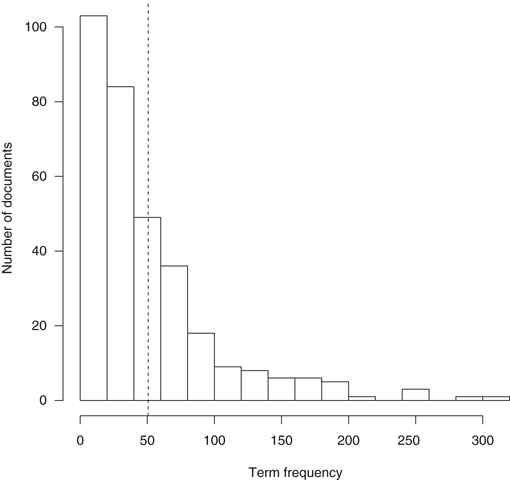
Once we lemmatize all three corpora and remove stopwords and non-relevant terms, the dimensions and sparsity of the document-term matrices is critically reduced, as observed in Table 5.3.5 The column called Original lemmas indicates the number of different terms of the lemmatized corpora, while Lemmas TFIDF shows the number of relevant terms selected considering TFIDF. In all three corpora, the number of terms is reduced to its half. Table 5.3 also shows the results of data reduction when we carry it out to a textual corpus containing all three previous corpora altogether. Note that the implementation of the TFIDF criterium in the “Whole” corpus produces a higher level of lemma reduction. The inclusion of the responses on all three issues (civil, on-call, and criminal) has an effect on the heterogeneity of the “Whole” corpus, which in turn reduces the number of discriminating terms within the documents. As shown in Fig. 5.1, now most documents have on average a small number of very relevant terms (the dotted vertical line marks the mean number of terms per document). We now have clean data ready to be analyzed in the rest of the chapter.

A309690_1_En_5_Fig1_HTML.gif


Fig. 5.1
Distribution of term frequency among all the documents in the whole corpus


5.3 On-Call Service as a Professional Problem (Hypothesis 1)


As explained above, judges who have recently finished their courses at the Judicial School start their professional career in Courts of First Instance and Magistrate. Findings in organizational decision theory and behavioral decision making suggest that the decision-maker adapts to a problem environment shaped by a number of organizational constraints.

Empirical findings related to Spanish junior judges suggested that on-call periods are specially problematic to junior judges during their 1st years. Regarding our first hypothesis, we aim at testing whether the differences betweeen civil, criminal, and on-call problems are significantly different from each other. These differences should arise because when asked about their main problems during civil procedures, criminal procedures, and on-call situations, judges refer to different things in each case. To carry out a systematic comparison of documents, we adopt a double strategy of analysis that involves both a classification and a scaling procedure.

On one hand, the hypothesis involves a simple classification problem—the identification of homogeneous groups of documents. In particular, we aim at testing whether the three different textual corpora constitute three different, homogeneous sets of textual data, different from each other.

On the other hand, we also aim at representing and explaining any structure or pattern in the (dis)similarities between (groups of) documents, in a way that the proximity between clusters and documents can be analyzed.

To do so, first, in order to obtain similar groups of documents based on the similarity of their vector representations, we will implement a hierarchical clustering algorithm and the results will be discussed. Second, a Multidimensional Scaling (MDS) algorithm will be used to scale the documents so that similarity between documents and clusters can be tested.


5.3.1 Method: Document Clustering and Scaling


The unprecedented growth of available textual data, either on the World Wide Web or in digital archives from publishers, governments or companies, has made of text mining a basic toolkit to “help people better understand and make use of the information in document repositories” (Srivastava and Sahami 2009). Among text mining techniques, Cluster analysis and Multidimensional scaling are now key methods for data grouping and classification, widely used in all kinds of data-intense scientific endeavors, such as market segmentation (Mooi and Sarstedt 2011), population cluster identification through genetic similarity (Witherspoon et al. 2007), analysis of political and legal data (Jakulin 2007), and information retrieval (Srivastava and Sahami 2009).

On one hand, a clustering algorithm divides a collection of documents into a set of similar documents, or clusters, so that “documents within a cluster should be as similar as possible; and documents in one cluster should be as dissimilar as possible from documents in other clusters” (Manning et al. 2008). This allows not only reducing large amounts of information to a small set of coherent elements, but its output can also be further used to train machine learning algorithms with various purposes such as automatic information retrieval or information extraction (Huang 2008). On the other hand, Multidimensional scaling (MDS) is an effective exploratory data analysis tool—used in various domains such as psychology (Jaworska and Chupetlovska-Anastasova 2009), political science (Lauderdale and Clark 2012), or text visualization (Fortuna et al. 2005)—to handle and visualize multidimensional data into a lower dimensional space, so that inferences can be drawn from the representation of the similarities between objects.

Note that both methods require a definition of what is for two documents (vector representation) to be “similar”. Instead of the commonly used Euclidean distance metric, we use the Bray-Curtis dissimilarity measure (Bray and Curtis 1957). Although Euclidean distance is very common in all kinds of clustering applications due to its more “natural” flavour (it can be conceptualized as “distance”, Greenacre 2005), it works well with ratio or interval data (Mooi and Sarstedt 2011) but not with count data. For count data (term frequencies), the Bray–Curtis dissimilartiy measure (Bray and Curtis 1957) is most adequate and is often used in ecological studies to account for clustering species based on species abundance in different sites (Greenacre 2005), although it has been also used and recommended in some NLP applications under certain conditions (Paukkeri 2012).

The Bray–Curtis distance metric between documents X and Y is


$$\begin{aligned} {d(X,Y)} = {{\sum_{i=1}^n |x_i - y_i|} \over{\sum_{i=1}^n (x_i + y_i)}},\end{aligned}$$

where x i and y i are the frequencies of the i th term in documents X and Y, respectively. Note that dividing the absolute value of the differences between frequencies by their sum, we always obtain a value between 0 and 1, which is a nice feature for a dissimilarity measure. A dissimilarity matrix is created for the 330 documents of our whole corpus using the vegan R package (Oksanen et al. 2013).

The clustering method that best suits our objectives is Hierarchical Agglomerative Clustering (HAC) (Manning et al. 2008). First, compared to other clustering methods (e.g., flat clustering methods such as k-means), hierarchical clustering does not require the previous specification of a desired number of clusters. Second, the output of the hierarchical method is highly informative in so far it delivers a hierarchy of high-quality clustered elements (Sandhya and Govardhan 2012). Typically, HAC starts out considering each document as one single cluster “and then successively merges pairs of clusters until all clusters have been merged into a single cluster that contains all documents” (Manning et al. 2008). This “nested sequence of partitions” (Sandhya and Govardhan 2012) is carried out on the dissimilarity matrix of all the documents. In order to minimize the within-cluster variance we use Ward’s minimum variance method (Ward 1963).6 On the other hand, the Multidimensional scaling (MDS) will handle the dissimilarity matrix of pairs of documents and reduce it to a low-dimensional representation so that dissimilarities among documents is preserved. Therefore MDS will deliver the relative positioning of our documents according to their similarity.7 Note that we use the tool here both as an exploratory data analysis method to observe structural patterns within our data, and as a check to the clustering analysis output. In order to achieve a precise understanding of the underlying structure of the data, only two embedding dimensions are specified (Borg and Groenen 2005).8


5.3.2 Results


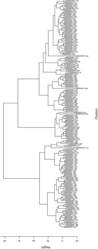
Figure 5.2 shows the results of the hierarchical clustering with a dendrogram of the whole corpus of judges’ descriptions of the main problems encountered during civil and criminal procedures, and on-call situations. Starting at the upper level of the tree, the method subdivides the documents into two main branches, each of which is in turn subdivided into two subbranches. Therefore, it is advisable to look at the clusters in a middle level of partition (i.e., at a proximity or height of between 2 and 3), since further down the tree the method starts creating too small clusters.

Moreover, given the source of our documents (three different questions in the questionnaire), we would expect to have three different clusters within which documents should be most similar to each other and most dissimilar with respect the documents in the other clusters. Therefore, we cut the tree so that we have three different clusters—that is, at a level of proximity (height) of 3 in the dendrogram.

A309690_1_En_5_Fig2_HTML.gif


Fig. 5.2
Dendrogram representing the results of the hierarchical clustering algorithm on all documents


Table 5.4
Distribution of the clusters within each type of documents. The results should be read as row percentages of documents


Cluster 1

Cluster 2

Cluster 3

Total

Civil

92.79

0.00

7.21

100

On-call

2.73

33.64

63.64

100

Criminal

19.27

3.67

77.06

100

In order to further explore the clustering results, we cross the content of each cluster against the actual source of each document (civil, criminal, or on-call). Table 5.4 shows the share of clusters within each type of document, while Table 5.5 accounts for the distribution of each type of document within each cluster. We observe two distinct phenomena. First, more than 90 % of the documents regarding civil problems have been classified into the first cluster, which points to the fact that problems related to civil procedures are highly specific and distinct from any other kind of problem. On the other hand, problems during on-call situations and problems regarding criminal procedures are less easily distinguishable. Although cluster number 3 contains a large share of both types of documents, the second cluster also contains one third of the on-call problems.


Table 5.5
Distribution of each type of document in each cluster. The table should be read as column percentages of documents


Cluster 1

Cluster 2

Cluster 3

Civil

81.10

0.00

4.94

On-call

2.36

90.24

43.21

Criminal

16.54

9.76

51.85

Total

100

100

100

This would point to the idea that while civil procedures raise doubts and problems of a very specific nature, there are commonalities between some of the problems related to criminal procedures and the ones raised during on-call situations. According to what we explained before in this chapter, this is hardly surprising, since most of the issues dealt with during on-call situations are regarding criminal matters. Table 5.5 helps depicting this relationship between these two types of documents. From the distribution of each type of document within each cluster we observe that the first two clusters seem to be distinctively thematic, the first one containing mostly civil issues, and the second one being overwhelmingly restricted to problems raised during on-call situations. The third cluster contains a fair share of both on-call and criminal issues, which would point to the overlapping areas in which problems during on-call situations could also be described as problems regarding criminal procedures.

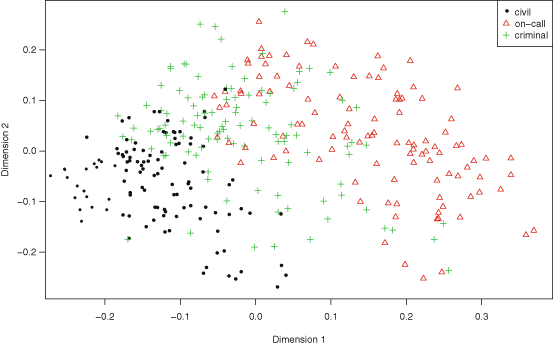
The extent to which, as clustering suggests, on one hand, civil procedures pose significantly different kinds of problems, and, on the other hand, criminal procedures and on-call situations trigger problems that occupy both overlapping and non-ambiguous areas of expertise, can be further tested when we apply a scaling method (MDS) to our set of documents so that we can both better visualize the results and use the method output to carry out further analyses.

A309690_1_En_5_Fig3_HTML.gif


Fig. 5.3
Representation of the positions of all the documents through multidimensional scaling. Different symbols account for the three different types of documents

Figure 5.3 represents the relations of similarity among all documents in just two dimensions. To ensure visualization we plot each type of document (civil, on-call and criminal) using different symbols. Note that documents lay nicely along the axis representing the first dimension showing a clear scale pattern. Substantive interpretation of the dimensions provided by scaling methods is fraught with dangers (Buntine and Jakulin 2006). In particular, when data are reduced into just a few latent variables (as we do with any scaling method by definition), we have no straightforward way to substantively interpret the components.

However, the results show a continuous scale—which we may safely call “dissimilarity scale”—from documents relating problems during civil procedures (far left) up to documents depicting specifically on-call problems, where documents on each extreme point of the scale are most dissimilar. Problems relating criminal issues lay in the mid section of the scale.

A309690_1_En_5_Fig4_HTML.gif


Fig. 5.4
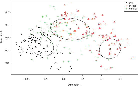
Representation of the positions of all the documents through multidimensional scaling and clustering results. Different symbols account for the three different kind of documents, and ellipses represent the three clusters

Although there is some overlapping between the documents from the criminal corpus with the other two types of documents, MDS provides us with a quite clear distinction between each type of document. This is still more apparent in Fig. 5.4, in which we have added ellipses representing the clusters previously obtained.

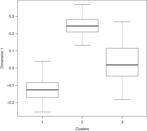
As we expected, clusters 1 and 2 mostly contain documents of just one type (civil and on-call, respectively), while cluster 3 represents an overlapping area between problems during on-call situations and criminal procedures, that is, the intersection between both sets of problems. Additionally, Fig. 5.5 shows the distribution per cluster of the values of each document in the first dimension provided by the Multidimensional scaling algorithm, showing a sharp separation between positions of documents in clusters 1 and 2, while documents in cluster 3 are move spread along the dimension, with the median position very close to zero (0.02).

A309690_1_En_5_Fig5_HTML.gif


Fig. 5.5
Boxplot representing the distribution of the scores of the first dimension of MDS for each of the four clusters

Finally, we test the effect of the type of problem and the membership of a document in a cluster on that document’s position in the scale. To do so we fit an Ordinary Least Squares regression model using the position of the document in the first dimension of MDS as outcome and the type of document and the clustering category as predictors. Note that the outcome variable (the position of the documents on the MDS first dimension) has both positive and negative values, denoting positions more to the right (positive) and left (negative), respectively. Results are shown in Table 5.6.

Model 1 in the table shows only the effect of the type of document on the position in the scale, using the civil type of document as the reference category. Note that the model predicts that both the on-call and criminal types of documents will have positive and significantly different positions in the scale than the documents depicting problems raised during civil procedures. Moreover, documents pertaining in the on-call corpus show higher positive values than those in the criminal corpus, indicating that, on average, these will be farther on the right side of the scale, while the coefficient for the criminal documents is smaller.


Table 5.6
Ordinary least squares regression results of the multidimensional scaling method on the results of hierarchical clustering


Model 1

Model 2

Model 3

(Intercept)


$-0.13 ^*$


$-0.12 ^*$


$-0.13 ^*$
 
(0.01)

(0.01)

(0.01)

[Ref. Civil corpus]
     

On-call corpus


$0.28 ^*$
 

$0.15 ^*$
 
(0.01)
 
(0.02)

Criminal corpus


$0.11 ^*$
 

$0.05 ^*$
 
(0.01)
 
(0.01)

[Ref. Cluster 1]
     

Cluster 2
 

$0.37 ^*$


$0.24 ^*$
   
(0.02)

(0.02)

Cluster 3
 

$0.16 ^*$


$0.08 ^*$
   
(0.01)

(0.01)

N

330

330

330

R 2

0.60

0.65

0.74

Resid. sd

0.09

0.09

0.08


Standard errors in parentheses

*indicates significance at p < 0.05

In a similar way, Model 2 shows the effect of a document being in a specific cluster on the posistion it occupies on the scale, with cluster 1 (the “civil cluster”) as the reference category. The results are similar in both the coefficients and their significance. Again, for a document being in cluster 2 (the “on-call cluster”) the model predicts a significantly different and positive position on the scale compared to documents within the “civil cluster”, while documents in corpus 3 will present on average smaller coefficients, though positive.

The two predictors are brought together in Model 3, where the same conclusions largely hold. On one hand, despite a potential collinearity problem caused by the inclusion of both predictors, all coefficients preserve reasonable values and remain significant. On the other, the fit of the model overall improves. While the models including the type of document and the cluster category separately were able to explain between 60 and 65 % of the variation in the data, the inclusion of both predictors raises the model’s goodness of fit to 75 % and lowers its residual standard deviation.9

The models, therefore, seem to provide evidence of the significant differences among documents, although these differences are only clear between problems triggered by civil procedures and the rest of the documents, while the distinction between criminal and on-call documents deserves a separate analysis.

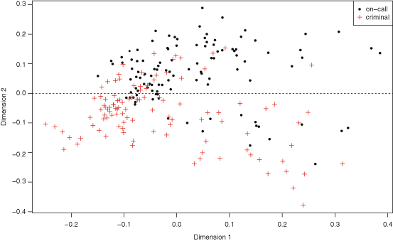
In order to explore the relationship between problems from criminal procedures and from on-call situations, we replicate the Clustering analysis and the Multidimensional scaling with only those documents. The results of the Multidimensional scaling in this separate analysis are shown in Fig. 5.6, that plots the results of Multidimensional scaling only on documents from the on-call and criminal corpora.

While differences here are not as apparent in one single dimension as those shown by documents pertaining to the civil corpus when the three corpora were taken into the analysis, here differences between the two types of documents seem to be in both dimensions. On the first dimension, documents depicting problems from ordinary criminal procedures tend to lay on the left side, while problems triggered by on-call situations are more on the right. On the other hand, most documents from the criminal corpus tend to be below zero in the second dimension (marked with a dotted line in Fig. 5.6), while most of the documents from the on-call corpus have positive coordinates on the second dimension.

A309690_1_En_5_Fig6_HTML.gif


Fig. 5.6
Representation of the positions of all the documents through multidimensional scaling. Different symbols account for the three different types of documents

In order to test the differences between both types of documents in both dimensions, we fit an OLS regression model to predict the position of documents in each of the two dimensions delivered by the scaling algorithm. Again, we use the type of document and the clustering results as predictors, although each of them now has only two categories.


Table 5.7
Ordinary least squares regression results of the multidimensional scaling method on the results of hierarchical clustering of the documents coming from the criminal and on-call corpora


Type of document
 
Cluster
 
Both predictors
 
Dim. 1

Dim. 2

Dim. 1

Dim. 2

Dim. 1

Dim. 2

(Intercept)


$0.03 ^*$


$0.07 ^*$


$0.14 ^*$


$-0.03 ^*$


$0.17 ^*$


$0.03 ^*$
 
(0.01)

(0.01)

(0.01)

(0.01)

(0.01)

(0.01)

[Ref. On-call corpus]
           

Criminal corpus


$-0.06 ^*$


$-0.13 ^*$
   

$-0.05 ^*$


$ -0.14 ^*$
 
(0.02)

(0.01)
   
(0.01)

(0.01)

[Ref. Cluster 1]
           

Cluster 2
   

$-0.20 ^*$


$0.05 ^*$


$-0.20 ^*$


$0.06 ^*$
     
(0.01)

(0.02)

(0.01)

(0.01)

N

219

219

219

219

219

219

R 2

0.07

0.30

0.55

0.03

0.59

0.34

Resid. sd

0.12

0.10

0.08

0.12

0.08

0.10


Standard errors in parentheses


$^*$
indicates significance at 
$p<0.05$

Results in Table 5.7 show that differences between documents from criminal procedures and on-call situations are significantly different in both dimensions, although these differences are smaller on average than what we found in the model including the three corpora.

An interesting feature of the model, though, is that each predictor seems to perform well in one dimension but not on the other. In particular, the first two columns show the effect for a document from the criminal corpus on its position on each dimension compared to the position of the documents from the on-call corpus. We may observe that the average difference in position between documents of both corpora are larger when taking into account the second dimension. On the contrary, when the predictors are the clusters (columns 3 and 4 of Table 5.7), the coefficient is larger when the outcome variable is the position in the first dimension.

Moreover, the model including the first dimension shows a much better goodness of fit with the clusters as predictors (both in R 2 and standard error of the model), while the one with the second dimension as outcome is better fitted when predicted by the type of document.

Results, therefore, give support to our first hypothesis in two different aspects. On one hand, when all the documents are considered, the specific and distinct features of the problems triggered by civil procedures stand out in a significant way, while the classification methods used are not able to clearly distinguish documents containing problems of criminal nature and raised during on-call situations. On the other hand, when only these latter two types of documents are taken into account, smaller but still signficant differences between the criminal and on-call problems are identified.

We now turn to our second hypothesis—the exploration of the distinctive problems raised during the operation of the on-call service.


5.4 Mapping Problems Through Topic Modeling (Hypothesis 2)


In our second hypothesis we aim at exploring the role of the outer environment (the organization) into the decision-making process of junior judges. In particular, we address the extent to which most problems and doubts faced when judges are on-call constitute demands from their organizational environment, and therefore merely procedural and behavioral, in contrast with a more theoretical-based nature of the problems raised during ordinary criminal, and specially civil, procedures. Should this be the case, solutions to these problems would not be contained in the corpus of legal knowledge judges acquire either in the law degree or preparing the entrance examination: theoretical legal knowledge.

Only gold members can continue reading. Log In or Register to continue