Recreating the Profit and Loss Account of Voyages of the Distant Past
Chapter 10
Recreating the Profit and Loss Account of Voyages of the Distant Past
Andreas Vergottis*
William Homan-Russell**, Gordon Hui‡ and Michalis Voutsinas‡‡
1. Introduction
The study of historical freight rate fluctuations over the previous two centuries has attracted the attention of several economists both maritime and non-shipping specialists. The nature of these studies varies and could be sub-divided in descending order of profusion into:
- long term shipping productivity gains and associated secular fall in across the board ocean freight rates;
- single route specific studies;
- the nature and periodicity of cyclical fluctuations;
- construction of freight rate indices;
- the contribution of falling freight rates to the reduction in barriers to trade;
- returns on capital to shipping investors; and
- port productivity trend developments
The literature is growing at exponential rate yet in certain respects the accumulation of knowledge at times resembles more a “Copernican” lens approach. It sorely lacks a “Newtonian” methodical tidying up system. The appendix contains a non-exhaustive list of such studies. However, in spirit the closest pro-genitor of the present one, is Lewis (1941), which to our knowledge has never been referenced in the subsequent shipping literature.
Empirical investigations have been constrained by the nature of available data with the lowest hanging fruit collected first. In general data on freight rates proliferate. This has encouraged several studies of type (a), (b), (c), (d) and (e) above.
Contrary to this, data on shipping profits is scant hence type (f) studies are rare. In theory one could recreate the profit and loss account of a benchmark ship by using a bottom up approach. Here the economic historian starts with the easily available freight rate data. He then makes certain deductions for costs and divides by the length of the voyage in days to arrive at a measure of unit profit. However, the input requirements of sufficient accuracy through the various steps are very stringent. Thus, to our knowledge, only Davis (1957), Evans (1964) and Vergottis (2005) have attempted such a task for the periods 1670–1730, 1850–1860 and 1950–1974 respectively. An alternative approach is to unearth historic actual voyage accounts. Here Kaukiainen (1990) is the prime example but a rather solitary one. The third alternative, is a detailed analysis of the market performed by an industry expert of the bygone era who had full command of the facts. This is in contrast to the economic historian of today who tries to recreate the puzzle from fragments of surviving information. Such a jewel of expert witness analysis, is equally rare but Allen (1855), provides a thorough and exhaustive evaluation of the Tyne/London collier route and the comparative advantage of steam versus sail in that market.
Furthermore, historical analysis of port productivity trend developments of type (g), are also extremely rare and sketchy. This is despite certain valiant efforts notably by North (1968). Where they do exist they tend to be of descriptive rather than quantitative nature, as the required time series data is hard to assemble.
Archaeologists can infer the existence of cities, their economic activities, trading links, wars etc from little more than pottery shreds. In our case the existence of freight rate data, which generally is very good, represent the pottery fragments. These can be used to “unearth” the complete picture of the centuries old tramp ship operator economics and their time charter equivalent profits (“TCE”), relating to voyages of the distant past. Accordingly this article presents a hitherto unutilised fourth alternative to shed light on the darkest areas of shipping literature, dealing with profitability of ships and port productivity developments of the distant past. This alternative is a cliometric model which utilizes a multi-route network top down approach. Here the inter-relationship of freights over the cycle is analysed in tandem, across several route arteries of the chosen network. The network cliometric top down approach makes use of the cardinal rule of tramp shipping. According to this rule, arbitrage forces quickly equate the daily time charter equivalent earnings of all routes for ships of the same type, engaged in them simultaneously.
In the case of a stable network of routes where, as first approximation, vessel speed is treated as given over the cycle, the tramp arbitrage law results in a cliometric system of linear equations of disarming simplicity. All that is required is:
- minimum of two export outlets combined with two import destinations;
- synchronous freight rate observations across the 2×2 network at two distinct points in the cycle, say “cycle low” and “cycle high”.
These eight freight rate data points can mathematically reveal the hidden profit and loss of the tramp arbitrageur in all its essential details route by route including the following hitherto unknowns:
- port turnaround time;
- vessel and cargo related port charges as per “custom of the trade”;
- time charter equivalent profit.
This is done with the minimum of knowledge regarding the commercial characteristics of the representative tramper, such as cargo capacity, speed, fuel consumption and bunker prices. Freight rate and bunker price data are generally readily available. The skeleton commercial specification of the typical tramper of various eras is also generally known.
Moreover, the implied system of linear equations is recursive and can be solved first for port turnaround time, then for port charges and then for time charter equivalent profit. This holds the promise that the most obscure subsets of shipping literature may be illuminated by taking a methodical top down cliometric tramp arbitrage approach. It also suggests the potential for new insights across the whole spectrum of maritime economic history. It helps to tidy up and systematize several strands of shipping research.
Armstrong (1993), highlights the risks of using inferred data as substitute for the raw original. Parallel to cliometric approaches such as the one suggested in this article, the more stringent and time consuming process of searching for lost original data should be pursued. Modern IT technology holds the promise that one day such data on port turnaround performance may be “unearthed”, collated and analysed. However even then there would be certain risks in linking recorded freight rate time series to observed vessel port turnaround performance measurements. On the one hand, in tramp shipping, the recorded freight rate time series reflects what was agreed in the loading and discharge clauses of a charter party. It does not necessarily reflect what was actually achieved by ships at the ports. Thus one needs to unearth old charter parties rather than port arrival and departure records. On the other hand, during sail ship days and early steamship era, such clauses often amounted to no more than the phrase “as per custom of the port”. To make matters worse, the sharing of terminal costs between shipowner and charterer varies and can be ad hoc from contract to contract. Once again this necessitates the tracing and analysis of the detailed wording of several clauses of very old and most likely untraceable charter party contracts. The cliometric top down approach presented here overcomes all these issues though the cautionary note of Armstrong is recognised.
In our view, the ideal approach should combine “easy to develop” cliometric calculations with “needle in haystack” efforts to retrieve original data. These can act as a reality check on each other and provide a framework for interpretation and analysis. In this spirit, at the end of this article, we go one step further and explore a bottom up analysis of tramp route profitability using all types of information and methodologies available to the economic historian.
1.1 The cliometric top down framework
Without loss of generality and in order to simplify exposition consider first the sailing ship era where cost of fuel was zero. The time charter equivalent earnings on any route are given by the following formula:

where:
E time charter equivalent earnings (“TCE”)
F freight rate per unit of cargo
C cargo size
T terminal charges at all ports involved
S total time in sailing/transit between all ports involved
P total time spent for queuing, loading, discharge at all ports involved
V defined as S + P: complete voyage duration
The cliometric investigation starts by noting that equation (1) can be reformulated as:

where:

Thus the freight rate of each route is made of two components. The first component α, is route specific and varies with the idiosyncratic port charges. The second component β*Ε, implies that all freight rates move up and down in tandem with the common time charter equivalent market rate. However, the β-sensitivity of each route to the broader market time charter earnings, is also idiosyncratic and reflects the voyage duration. In turn the voyage duration β, can be subdivided into a steaming time component and a port turnaround time element.
Our rudimentary cliometric model treats F, C and S as known inputs and then solves for the unkowns P, T, E and V. More sophisticated versions can be developed whereby the latter list of unknowns grows “at the expense” of the former list of known inputs.
In passing it is noted that equation (2) suggests that a freight rate index can be constructed by simply taking the arithmetic average of rates across several routes. The index then represents the theoretical freight rate for the network “average route”. The α of the index is the mean α of all the routes in the network, and thus captures the average port charges across all routes. Similarly, the index will capture the mean β of all the routes, representing average voyage duration.
1.1.1 Network stability
The notion of “regime change” and its opposite “network structure stability” is introduced here, before proceeding with the rest of the analysis. We define “network structure stability” as a situation where the parameters α and β in equation (2) remain stable over a certain period of time for a certain network of routes for each of its arteries of complete round voyages. In the case of the constant α, this will tend to hold true by the fact that port charges are tariff based and can remain unchanged for decades. In case of the slope co-efficient β, this will tend to trend lower with productivity changes in either or both the sailing speed of ships and/or their port turnaround times. Also the change of trade flows, the inversion between fronthaul and backhaul routes and the triangulation of previous singular routes imply “regime change”.
Both α and β have been reducing over the span of decades. However over a typical full cycle of say five years’ duration, may be considered as approximately constant. One should not naively make such an assumption. Fortunately “network structure stability” can be tested. This can be done either visually by plotting several freight rates on the same chart or in scatter plots. It can also be tested via econometric means. Regarding the latter, we note that equation (2) implies all freight rates in different arteries of the same stable network will be linearly related to each other. Hence a scatter plot of two freight rate time series should closely resemble a straight line in case of network stability. The cross-correlation matrix of the freight rates of all arterial routes should be populated with one not just on the diagonal but on all off-diagonal entries, in the absence of “regime change”. Off course in working with stochastic versions of the above equations one should tolerate certain deviation from the limiting pure ideal of 100% correlation and pure straight line scatter plot patterns.
“Regime change” is not necessarily bad for the econometric investigation. Normally it can be identified (e.g., the point when a fronthaul route reverts to backhaul status can be easily detected) and thus controlled for. It produces a richer set of equations recombining the same parameters. This can be exploited in order to calculate the unknown parameters with better statistical accuracy.
1.1.2 The cliometric mathematical system of equations
Given a minimum of two export outlets (“X” and “Y”) and two import destinations (“M” and “N”), the tramp arbitrage rule results in the following system of equations:
where:
Fxm reight rate on route linking export port X to import destination M
Txm = Tx + Tm; terminal charges at each end from export port X to import destination M
Sxm sailing transit time from export port X to import destination M (round voyage basis)
Pxm = Px + Pm; port turnaround time at export port X and import destination M
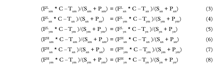
and similarly for other permutations of the subscripts. The superscripts L and H represent “cycle low” and “cycle high” observations.
At this stage we treat cargo size C as fixed across routes and through the cycle for the benchmark tramp ship just to simplify exposition. In the econometric application presented below this restriction is relaxed.
The recursive nature of the system can be exploited by taking the difference between “cycle high” and “cycle low” observations, which allows the unknown terminal charges to drop out of the picture.
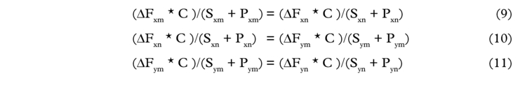
This results in three equations and four unknowns, the latter being the port turnaround times for the round voyages. To close the system equation (12) is added:

Equations (9)–(12) can be solved for the unknown round voyage port turnaround times.
The next step involves taking either equations (3)–(5) or (6)–(8) and adding the following equation (13) to close the system and solve for terminal charges:

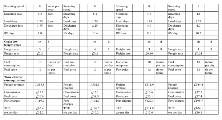
Finally time charter equivalent earnings E can be calculated for any stage of the cycle, as all the formerly unknowns that enter a round voyage TCE calculation have been solved for.
In case where there are more export and import points than the simple 2×2 network described above, the resulting system of linear equations is over-determined. A subset of equations suffices to solve for the unknowns. In econometric analysis using stochastic versions of the equations, it offers the advantage of using additional information to derive results and stress test them for accuracy and robustness through statistical means.
Moving on the steamship era, the cost of bunkers has to be factored into equation (1). The engineering technology of representative trampers is well recorded. Harley (1970) provides a succinct summary. Consumption of bunkers for a given speed of the benchmark tramp ship is documented and considered as known input number in our cliometric model. Price of bunkers is also readily available. Hence the bunker cost per tonne of cargo carried can be calculated. For ease of computation, the imputed bunker cost per tonne is deducted from the recorded freight rate per tonne. Thus “net of bunkers freight rates” are derived. The rest of the analysis can then proceed precisely as has been presented above for the sail ship era. Once again more sophisticated cliometric models can be developed which solve for bunker consumption and speed rather than treat these as assumed known inputs.
1.2 Case study: the Northern European coastal coal freight market 1848–1936
The Northern European coastal coal freight market represents a neat compact network of routes to apply the various methodologies described above. The two main export outlets are Tyne (Newcastle, Blyth, Wear) and Wales (Cardiff, Swansea). The main import destinations are London, Hamburg, Havre, Rouen, Caen, St Malo, Dieppe, Honfleur and Brest. It is well known that shipping coal out of the main export UK outlets to nearby UK/North European ports was predominantly a one way market. Tramp coasters departed from Tyne or Wales loaded with coal, discharged their cargo in nearby destinations and ballasted back to the load ports empty.
Some routes are more liquid than others and offer more regular and complete freight rate time series. Weekly freight rate data with certain gaps have been assembled for the period 1848 to 1936. For the purpose of this study and subsequent investigations around 42,000 freight rate data points were collected spanning almost a century of cyclical swings and trend developments. The process of data collection is ongoing.
1.2.1 Historic backdrop 1848–1936
At the beginning of our overall study the 300 tonne collier sail ship reigned supreme. In summer 1852 the first 650 dwt tonne steamer was introduced in the Tyne/London route. After minor teething problems, the concept quickly proved successful. Thus by 1870 steamers had practically displaced the sailing collier in many of the Northern European coastal routes. The size of coastal steamers increased progressively with about 1,000 dwt tonnes being the representative tramper during the period 1880–1900. The average size of coastal collier increased rapidly after the turn of the nineteenth century with 1,450 dwt vessel becoming the benchmark coastal tramper by 1910. By 1936, a combination of economic, industrial and political factors resulted in severe shrinkage of the North European near-sea coal freight market. This delineates the end of our investigation period.
1.2.2 Preliminary tests of network stability
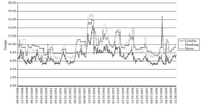
The simple tramp arbitrage model suggests that freight rate observations on a basket of routes that are part of stable network should be 100% correlated with each other. Starting with the sail ship era, Figure 1 shows the freight rate patterns for three of the major routes during the period summer 1848 to winter 1859. If there is a flaw in the conceptual model, a simple chart would normally reveal it easier than “black box” computations.
The figure highlights the close correlation between the various routes during the sail ship era. It also shows that the London short haul route has a low beta as one would expect given that the slope coefficient, against the unobservable common time charter equivalent, is proportional to voyage duration.
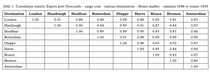
Numeric correlations are provided in Table 1 below. The tramp arbitrage model suggests that not only the diagonal but also the non-diagonal entries should not differ materially from 1.
It is recommended that correlations should be computed over periods that include at least one full cycle. Correlations computed around a period where the market is constantly at a flat low would fail to shed light on the underlying stability, or lack thereof, of the network. Typically during cycle lows, freight rates and the unobservable TCE remain totally flat, with TCE “stuck” at around operating cost level. Thus the whole of the recorded variance taken during a protracted cycle low would be “noise”.
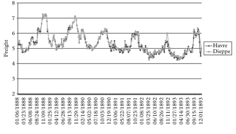
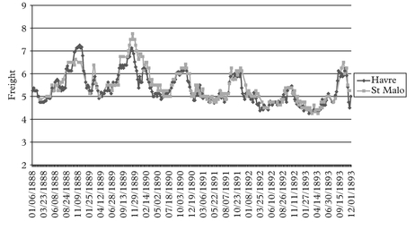
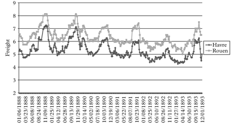
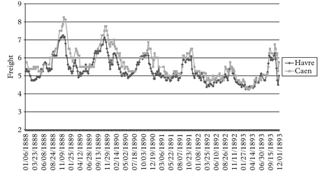
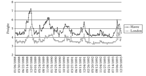
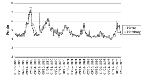
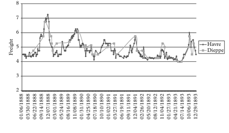
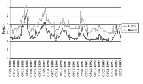
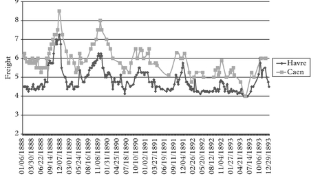
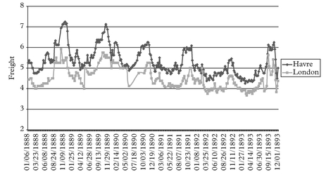
Moving to the steamship era, we tend to observe a boom at the turn of each decade. All these booms look very much alike with each other in terms of their main features. We show the detailed figures for the full cycle Jan 1888 to Dec 1893 period, being very representative of the patterns observed in all other steamship full cycle periods around the turn of each decade.
We have grouped the various freight rate plots under different permutation schemes. For practical purposes the first thing to identify before plotting the charts is the most liquid route, in the sense that it has the fewest observation gaps in the series. This we
call the benchmark route. For the outbound routes from Tyne the destination to Havre is our chosen benchmark route. For the outbound routes from Wales the same destination Havre is chosen as the benchmark route.
The charts have been grouped as follows. Figures 2–7 plot each of the outbound routes from Tyne against the benchmark Newcastle/Havre route. Figures 8–13 plot each of the outbound routes from Wales against the benchmark Cardiff/Havre route. Finally Figures 14–20 pair together each destination with the two export outlets Newcastle and Wales. All figures are in shilling per tonne and the freight rates have been computed net of bunkers.
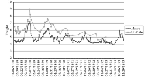
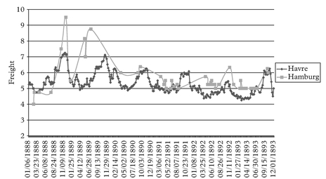
Note: The Cardiff/Hamburg route is illiquid. Hamburg is primarily served from Newcastle