Fleet Operations Optimisation and Fleet Deployment – An Update

Chapter 21
Fleet Operations Optimisation and Fleet Deployment — An Update
Anastassios N. Perakis*
1. Introduction
Optimising the operation (i.e. minimising operating costs, if revenues are fixed) of a single merchant ship is not difficult to do and can be achieved by a few simple calculations, which can point out the minimum of the operating cost curve as a function of the speed, for example. Texts such as Stopford1 can provide useful info on the above. Optimising an entire fleet of generally different ships, however, is definitely not as simple, and requires certain levels of computer, probability, optimisation and other mathematical skills, as we will see in the following.
Deployment of merchant shipping fleets covers a wide range of problems, concerned with fleet operations, scheduling, routing, and fleet design. Many use some kind of economic criterion such as profitability, income or costs on which to base decisions. (Benford,2 Marbury,3 Fischer and Rosenwein,4 and Perakis 5). Others use non-economic criteria such as utilisation or service; these are more common in fleet deployment models used in the liner trades.6 Reviews of various fleet deployment models and problems are given in.Ronen,7 Ronen,8 and Perakis.9
An aspect of fleet deployment not covered extensively in the literature until the early 1980s was “slow-steaming” analysis and optimisation. “Slow steaming” is the practice of operating a ship or fleet of ships at a speed less than design or maximum (sustained) operating speed, in order to take advantage of improved fuel economy and reduced operating costs, but, most importantly, to reduce fleet overcapacity (if done by a large number of ship owner).
Managers of merchant ship fleets, especially bulk carriers and tankers, frequently find themselves with excess transport capacity, and hence must decide which ships to use (and at what speeds) and which to keep idle (or perhaps make available to another fleet by sale or charter). Moreover, if fuel prices become relatively high, excess transport capacity offers the potentially profitable strategy of slow steaming some or all of their ships. Such a strategy not only substantially reduces the operating costs of the fleet, but furthermore reduces the supply of tonne-miles of the existing total bulker fleet, thereby improving the depressed freight rates. On the other hand, a sharp drop in fuel prices could make it advisable to “fast-steam” ships built during the expensive fuel era, although this would be limited by their design speed and associated operating margin.
The remainder of this chapter is organised as follows: Section 1 discusses the correct solution of a simple fleet deployment problem, which has been earlier suboptimally solved in the literature. It is shown that its correct solution can save over 15% of the annual fleet operating costs, or $7.93 million per year, for the same 10-ship fleet of the previously published example. In Section 2, more realistic, single-origin, single-destination, and even multi-origin, multi-destination fleet deployment problems for (liquid or dry) bulk shipping are formulated and solved, using both nonlinear and a series of linear programmes. In Section 3, fleet deployment problems for Liner Shipping Fleets are solved, and specific examples are given from the fleet of a major liner company. Section 4 provides a summary and conclusions, as well as recent developments in this area. An alphabetical list of references is given at the end of this chapter.
2. A Simple fleet Deployment Problem
The ships of a fleet could be assumed to belong to N different groups, each consisting of n(i) sister ships, i = 1, …, N, of equal cargo carrying capacity, speed and fuel consumption (or in general, operating costs). Design speed, cargo capacity and operating costs will in general be different among different ship groups. This is both an efficient and general model, since the case of no two ships in a fleet being identical is obviously covered by setting n(i) = 1, i = 1, …, N. The mission of a fleet is assumed, for our purposes, to be the movement of one commodity between two given ports.
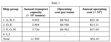
A simple (but realistic) bulker fleet deployment problem was defined in Benford (see endnote 2).Some of the assumptions inherent in the solution approach, such as no-cost lay-up of unneeded vessels, a contract to move a given quantity of a given commodity between one origin and one destination port, availability of more than enough ships (tonnage) suited to the trade, etc., were not unrealistic. However, the method proposed for its solution did not give the optimal answer, primarily because of an artificial constraint that all vessels must be operated at a speed resulting in the same unit cost of operation per ton of cargo delivered, imposed for ease of solution, but not a natural constraint of the problem. Table 1 below presents the approach adopted in Benford (see endnote 2) and its results.
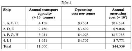
In Perokis (see endnote 5), the problem was correctly solved analytically, without the above equal unit cost constraint, using Lagrange multipliers. The results (see Table 2) showed an improvement of at least 15% over those of Table 1, thus verifying once more that ‘constraints impair performance.’ More realistic and complicated versions of the problem solved in that paper were subsequently formulated and solved.
Comparing Tables 1 and 2, we see an annual cost reduction of $7.93 million, or over 15%. This represents a considerable improvement. The difference in costs could be even greater if lay-up charges are levied against ships I and J in the solution presented in Table 1. On the other hand, this difference could possibly be reduced if ships I and J could be chartered or sold to a third party at a particular price.
Perhaps it is now appropriate to clarify that in the above problem, the annual demanded transport capacity is assumed to be a given output (constant). This is the case for vessels operating under relatively long-term charters, which normally specify, among other
things, the freight rate and the amount of cargo to be carried annually. In a normal market environment, long-term charters are the overwhelming majority of fixtures, whereas vessels operating in the spot market constitute less than 10% of the available capacity.
The conclusion from the above is that, in contrast to past practices where significant effort has been directed toward the optimisation of the design and operation of individual ships, an owner of a fleet of ships (usually non-uniform in terms of age, size and operating speed) should operate each ship in a manner generally quite different from that dictated by single-ship optimisation. Adoption of the results of this and subsequent research should result in significant cost savings in the operations of several shipping companies.
3. More Realistic Bulk Shipping Fleet Deployment Models
Perakis and Papadakis,10,11 and Papadakis and Perakis,12 presented far more realistic and complicated fleet deployment problems and their “optimal” solutions. The problem of single-origin, single-destination fleet deployment was first studied. A computer programme was developed to solve the problem and to help the fleet operator to make slow steaming policy decisions. A detailed discussion of the problem solution and a sensitivity analysis are presented in Perakis and Papadakis (see endnote 10). Sensitivity analysis provides the user with an understanding of the influence on the total fleet operating cost of its various components. For small to moderate changes of one or more cost components, the user can get an extremely accurate estimate of his new total operating cost without having to re-run the computer programme. Some interesting conclusions were made on the basis of the sensitivity results.
The fleet deployment problem with time-varying cost components was also formulated and solved. A computer programme was developed to implement the solution of this problem (Perakis, Papadakis and Pogoulates).13 The relevant algorithms are briefly described there as well. The problem of fleet deployment when the cost coefficients are random variables with known probability density functions was formulated in detail (see endnote 11), where analytical expressions for the basic probabilistic quantities were presented. A shorter description of the above is included in this presentation.
3.1 Objective function and constraints
A fleet, consisting of a given number of ships, is available to move a fixed amount of cargo between two ports, over a given period of time, for a fixed price. Each vessel in the fleet is assumed to have known operating cost characteristics. The problem objective is to determine each vessel’s full load and ballast speeds such that the total fleet operating cost is minimised and all contracted cargo is transported.
A first constraint imposes upper and lower bounds on the vessel full load and ballast speeds. These speed constraints are necessary to ensure a feasible solution to the problem; which is, that each speed is less than or equal to its maximum and greater than or equal to its minimum operating limits. In practice, the minimum speed is non-zero and is determined by the lower end of the normal operating region of the vessel’s main engine. The minimum speed should also be adequate for purposes of ship safety in maneuverability and control. The equality constraint must be satisfied to insure all contracted cargo is transported.
This formulation is based on the following assumptions, some of which use state-of-the-art empirical formulae taken from published articles, cited in the list of refs of the detailed papers and reports of ours (see endnote 10)14:
- A vessel carries a full load of cargo from load port to unload port.
- When the vessel is operating in restricted waters, it has a known and constant restricted speed which is usually the maximum allowable speed in the region in question, hence requiring a known, fixed power and fuel rate.
- The number of days a vessel spends in port per round trip is known and constant.
- The charges incurred at the load port and unload port per round trip are known and constant.
- The amount of fuel burned per day in the load port and unload port is known and constant.
- The annual costs of manning, stores, supplies, equipment, capital, administration, maintenance and repair, and make ready for sail are known and constant.
The power of vessel i (in HP) may be expressed by:
 for the full load and by:

for the ballast condition, where Xi and Yi are the full load and ballast speeds of ship i respectively and the rest are appropriate constants.
The all-purpose fuel rate for a fully loaded vessel i may be expressed by:
(Rf)i = gi·pi2 + si·pi + di for the full load and by
(Rf)bi = gbi · pbi2 + sbi · pbi + dbi
for the ballast condition where pi and pbi are the normalised (percent) pi and pbi respectively, and the rest are appropriate constants.
- The total annual cost of laying up vessel i is known for all i = 1, …, z.
- The number of days per year vessel i is out of service for maintenance and repair is known and constant.
- This problem formulation and solution is for a single stage, “one-shot” decision.
In the literature, the number of tonnes carried per year is assumed to be a linear function of a ship’s full load and ballast speeds. In our research, we have shown that this assumption can be quite unrealistic. This function is quite nonlinear in nature. A derivation of this function may be found in Perakis and Papadakis (see endnote 10).
Operating costs, developed in detail in Perakis and Papadakis (see endnote 14)15, are considered to fit into one of two categories, those that do not vary with ship speed, or daily running costs, and those that vary with ship speed, or voyage costs. Typical plots for the total (not per tonne) operating costs per year for a particular ship, for various ballast speeds, are given in Perakis and Papadakis (see endnote 10).
A typical plot of F(Xi, Yi) is also shown in Perakis and Papadakis (see endnote 10), as a function of the full load and ballast speeds. It is seen that F is a smooth convex curve or surface with a single minimum. There is also a finite speed range in which F is not very different from its minimum value, a property which allows approximate solutions to the problem using very different speeds for individual ships to produce total fleet costs very close to one another and to the optimum cost itself. For Xi and/or Yi going towards either 0 or 8, F approaches infinity. Figures 1 and 2 are for the same ship and for constant route data.
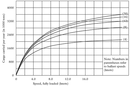
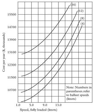
Figure 2: Typical plot for the total operating cost per year as a function of ship full load and ballast speeds
Introducing the linear inequality constraints on the speeds complicates the problem solution considerably. In the first part of this research, an External Penalty Technique (EPT) has been combined with the Nelder and Mead Simplex Search Technique to solve our optimisation problem. The purpose of a penalty function method is to transform a constrained problem into an unconstrained problem which can be solved using the coupled unconstrained technique.
A computer programme has been written to solve this problem using the techniques and the formulation mentioned above. The solution returned consists of the ship speeds, for those vessels specified for analysis, that will minimise the total mission operating costs and fulfil the cargo transport obligation.
For the lay-up option, it is shown in the technical report that for even moderate numbers of ships in a fleet, it is rather too time-consuming to use an exhaustive enumeration scheme. Instead, a dynamic programming-like sequential optimisation approach is developed, significantly reducing the computational burden. If Z is the number of ships in the fleet, the maximum number of fleets we will have to examine using this approach is Mmax = Z(Z + 1)/2 – 1. The actual number of fleets which we will have to consider will be significantly smaller than Mmax, due to the elimination of several fleets as infeasible and much smaller than the upper limit of total possible cases. The above scheme has been implemented and referred to in the following as the operating cost without re-running the programme. This property holds for a given fleet and not in cases when one or more ships are laid-up or chartered to a third party (on top of the changes in the cost components).
The fleet deployment problem with time-varying cost components was also studied. A time horizon in this formulation is any interval within which cost components are constant but at least one of them is different than its value in another interval. In other words, our cost components are given ‘staircase’ functions of time. In the case of rapidly changing costs, resulting in rather short intervals where these costs are constant, the problem of non-integer number of round trips per interval could be crucial. A heuristic approach was developed to find the nearest integer solution corresponding to the non-‘integer’ solution generally provided by the SIMPLEX algorithm.
Further details may be found in Perakis and Papadakis (see endnotes 10, 11, 15), and the associated user’s documentation, Perakis, Papadakis and Pogoulatos (see endnote 13), where a more extensive multi-page flow-chart is presented.
The fleet deployment problem for the case when some of the cost components are random variables with known probability density functions was finally considered (Perakis and Papadakis (see endnote 11)). We note that the minimum of the possible mean values of the total annual operating costs, Cmin and the variance of Cmin can be found relatively “easily”. However, this approach has not yet been implemented on a computer and probably will not prove very useful: The inputs to the problem (i.e. the user-supplied probability density functions) can have any particular theoretical or experimental form, thus discouraging the development of any general computer code for this problem.
3.2 The multi-origin, multi-destination fleet deployment problem
The problem of minimum-cost operation of a fleet of ships which has to carry a specific amount of cargo from several origin ports to several destination ports during a specified time interval was next examined. During the season any vessel can be loaded in any source port (S) and unloaded at any destination port (D) provided that these ports belong to a subset I or J (respectively) of the total set of ports, such that draft and other constraints for the corresponding vessel are satisfied. Under this assumption for each vessel the number of possible routes (number of possible sequences of S–D ports) is quite large. The full load and ballast characteristics of each ship on each route are assumed to be known.
This nonlinear optimisation problem consists of a nonlinear objective function and a set of five linear and two integer constraints. The objective function to be minimised is the total fleet operating cost during the time interval (shipping season) in question. The following constraints have to be satisfied:
- for each vessel, the total time spent in loading, travelling from origins to destinations, unloading and travelling from destinations to origins plus the lay-up time has to be equal to the total amount of time available for each ship in the shipping season,
- the total amount shipped to a particular destination j must be equal to the amount of cargo to be delivered to j during the shipping season (in tonnes),
- the total amount of cargo loaded from a particular source i must be less or equal to the cargo available at i,
- for each ship, the number of trips to destination j must be equal to the number of trips out of j,
- same as (d) for all source ports;
- the full-load and ballast operating speeds have to be between given upper and lower limits,
- the numbers of full load and ballast trips for each vessel, origin and destination combination must all be non-negative integers.
The constraints presented above are linear except constraints (a) and (g). The maximum number of unknown variables (if all source and destinations ports are accessible by any ship of the given fleet) is (4·I·J+1)·Z. The number of the associated constraints is 2Z+(1+J) (Z+1)+4·I·J·Z. For a case with I=4, J=6 and Z=10 we have 970 variables and 1,090 constraints. Using today’s personal computers, it is clear that we cannot use any classical nonlinear optimisation technique, since the expected computation time would be too long.
In the case of the multi-origin, multi-destination fleet deployment problem, it was seen that the linear programming approaches to the literature do not take into account significant nonlinearities of the relevant cost functions and may lead to very suboptimal decisions. The iterative procedure we developed uses a linear programming software in an algorithmic scheme that takes into account these nonlinearities and produces accurate results.