Emissions from Forest Fires: Methods of Estimation and National Results

(6.1)
The Seiler and Crutzen (1980) approach has been applied, after changes, refinements and integrations, to FE studies from global to local scale and for a variety of aims and purposes (e.g. Battye and Battye 2002; French et al. 2004; Narayan et al. 2007; Wiedinmyer and Neff 2007; Shultz et al. 2008; Wiedinmyer et al. 2010; Thonicke et al. 2010; Carvalho et al. 2011). A common element of these studies and applications is the analysis of uncertainties in the factors of the above mentioned Eq. 6.1. In particular, BA, EF, and F l have been pointed out by several Authors as the factors limiting the accuracy of long-term FE data sets (Peterson 1987; Peterson and Sandberg 1988; Battye and Battye 2002; Schultz et al. 2008). To represent their variability then becomes the challenge in FE inventories development (Langmann et al. 2009).
Large systematic errors in BA assessment may exist in relation to the reporting system (Peterson 1987). Barbosa et al. (1999), Korontzi et al. (2004), Al-saadi et al. (2008) analyzed the burnt area uncertainty and its effects of FE using different spatial datasets. New advances in remote sensing have made datasets of active fires and burned areas widely available, and have also provided temporal and spatial resolution improvements (Ottmar et al. 2009), but the presence of clouds or confused signals could strongly affect data (Stroppiana et al. 2010); Friedli et al. (2009b).
Fuel load (F l ) is considered as the source of the largest errors in FE estimates (Peterson and Sandberg 1988; Peterson 1987; Hardy et al. 2001), due to the large variability in ecosystem types and species composition. For example, Dimitrakopoulos (2002) pointed out the high variability of fuel load within Mediterranean vegetation, ranging from 4.85 t ha−1 in grasslands to 53 t ha−1 in evergreen sclerophyllous shrublands (fuel depth: 1.5–3 m). Recently, to obtain a better simulation of spatial variability in fuel load, several Authors integrated biochemical models (van der Werf et al. 2006) or dynamic global vegetation models (Thonicke et al. 2010) in FE inventories.
Peterson (1987) and Peterson and Sandberg (1988) demonstrated that EF variability (mainly due to type of pollutant, type and arrangement of fuel, and combustion efficiency, CE), contributes to about 16 % of the total error associated with emissions. The uncertainty is higher for compounds and biomes that have not been studied in detail (Langmann et al. 2009). Ward and Hardy (1991) suggested that EF could be better assessed considering the two phases of combustion, and then the fraction of biomass consumed by each process. The CE concept was then introduced, in order to involve the fractional rate of complete combustion. Values of CE exceeding 90 % indicate the flaming phase, while values lower than 85 % indicate smoldering combustion (Ward and Hardy 1991; Yokelson et al. 2007).
Another key component in the estimate of the amount and source of emissions (Ottmar et al. 2009) is the combustion completeness (CC, in %) (Shea et al. 1996). CC represents the ratio between consumed and available fuel load, and depends on fire type, fuel type and its moisture content (Ward et al. 1996; Battye and Battye 2002; Langmann et al. 2009). CC of coarse and wet fuels is lower than fine and dry fuels. Most FE estimation models determine combustion factors for each fuel strata (e.g. stems, leaves and litter) and moisture conditions, allowing for a detailed description of CC (e.g., Reinhardt et al. 1997; Hardy et al. 2001; van der Werf et al. 2006). In order to increase the level of accuracy for the assessment of CC, Chiriacò et al. (2013) integrated a methodology proposed by Bovio (2007) based on the level of damage assessed on the basis of forest vegetation class and scorch height, which depends on two main factors: the intensity of the fire and the type of forest vegetation affected by fire.
6.3 Description of Emission Factors for GHGs
According to Andreae and Merlet (2001), the mass of pollutant produced (Mx, in g) per mass of dry fuel consumed (Mb, in kg) is referred to as emission factor of a chemical species x (EF x ) (g kg−1), which translates biomass burned into trace species emissions (see Eq. 6.2).


(6.2)
Since the ’80s, a number of large projects dealing with biomass burning experiments and EFs have been coordinated in different ecosystems (Andreae and Merlet 2001). Most of these integrated projects focused on rainforest and savannas in Africa (e.g. Lacaux et al. 1995; Hao et al. 1996; Delmas et al. 1999; Swap et al. 2003) and Brazil (e.g. Crutzen et al. 1985; Kaufman et al. 1998; Yokelson et al. 2007). The mentioned field campaigns provided highly scattered information through the literature (Andreae and Merlet 2001); due to the different adopted methods of EF measurements, these data also present a large variability. In 2001, Andreae and Merlet reviewed and summarised EFs for a broad number of chemical species and for various types of biomass burning, such as savanna and grassland, tropical forest, extra-tropical forest.
Except for very few studies, there is a lack of available emission data from boreal zone and temperate forest, despite the importance of fire in these areas (Koppmann et al. 2005; Urbanski et al. 2009). Recently, Urbansky et al. (2009) compiled EF data for five broad vegetation cover types, considering temperate forest too. EF data from this ecosystem type mostly derived from experimental and prescribed fires in the United States and Canada, typically ignited under favorable weather and fuel conditions in order to manage low intensity fires.
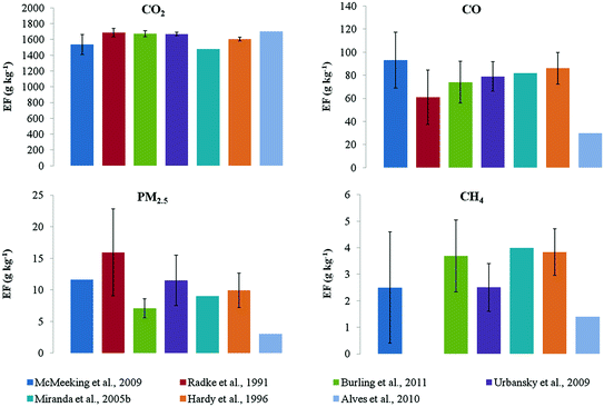
In Mediterranean areas, Miranda et al. (2005b) collected data of emission from shrubland experimental fires in the framework of the SPREAD project (Forest Fire Spread Prevention and Mitigation 2002–2005 founded by EGVI-2001-00027). More recently, Alves et al. (2010, 2011) detailed particle and trace gas EF for prescribed fires in Mediterranean shrubland and wildfires of the 2009 summer season, respectively. Fig. 6.1 compares several shrubland EFs for PM2.5, CO, CO2, CH4.


Fig. 6.1
Comparison among shrubland emission factors (g kg−1). Data derived from literature
6.4 Fire Emissions Modelling
According to Debano et al. (1998), quantitative predictions of fire effect models can be distinguished based on the fuel consumption modelling approach. Empirical models (McRae 1980; Brown et al. 1991; Prichard et al. 2005) use statistical relationships derived from measured woody fuel consumption data (Hollis et al. 2010) while physical models fully describe heat transfer processes (Albini 1976a). Semi-physical models result in the combination of these two approaches (Albini et al. 1995; Albini and Reinhardt 1995, 1997).
Up to now, among a conspicuous number of fuel consumption models, CONSUME (Fuel Consumption model, Ottmar et al. 1993, 2006) and FOFEM (First Order Fire Effect Model, Reinhardt et al. 1997) are those mostly used. CONSUME falls into the empirical model category, predicting fuel consumption by combustion phase, heat release and pollutant emissions (Prichard et al. 2005). FOFEM employs the physical model of heat transfer BURNUP (Woody fuel consumption model, Albini et al. 1995; Albini and Reinhardt 1995) to predict woody and litter fuel consumption and heat release.
At regional scale, Urbanski et al. (2011) presented the 2003–2008 Wildland Fire Emission Inventory (WFEI) in the contiguous United States. The product combines observation from satellite data, fuel loading maps, fuel consumption models (both COMSUME and FOFEM), and an EF database. Air pollutant emissions associated with forest burning in Texas were estimated by Dennis et al. (2002), based on survey and field data on area burned and land covered, and FOFEM for fuel consumption and emission factors.
At local scale, several case studies have been performed to determine the impact of fire events on air quality and identify the source of air pollution. Clinton et al. (2006) implemented FOFEM algorithms to quantify the source and composition of smoke and emissions from wildland fires that affected Southern California, USA, in October 2003. French et al. (2011) applied the two models to compare the different methodologies of FOFEM and CONSUME to estimate carbon loss from terrestrial biosphere resulting from wildland fires in Canada. Bacciu et al. (2012) applied FOFEM in Mediterranean areas, estimating type and amount of Mediterranean vegetation fire emissions from Sardinian fires (2005–2009), and compared 2005 emission estimates with the Italian Emission Inventory (NEI-PROV, De Lauretis et al. 2009) (Table 6.1).
Table 6.1
Average pollutant and GHG mass (Gg) by category from Sardinian fires (2005–2009)
YEAR | PM10 | PM2.5 | CH4 | CO | CO2 | NOX | SO2 | TOTAL |
|---|---|---|---|---|---|---|---|---|
Mean | 0.78 | 0.66 | 0.32 | 5.97 | 200.97 | 0.32 | 0.12 | 209.15 |
2005 | 0.41 | 0.34 | 0.16 | 2.98 | 0.18 | 0.07 | 4.14 | |
NEI-PROV | 0.62 | 0.62 | 0.34 | 3 | – | 0.09 | 0.03 | 4.74 |
6.5 Fire Emission Historical Trends and Future Scenarios
A crucial point to support emissions inventories and modeling of air quality and climate change issues has been recognized in up-to-date, accurate, and consistent FE estimates (Battye and Battye 2002; Granier et al. 2011). In addition, the spatial distribution pattern quantification is decisive for several applications, including air quality management plans, and emission source models coupled with dispersion models and decision support systems (Bacciu et al. 2012).
Over the past decades, a number of inventories, both at global and regional scale, were developed to estimate gaseous and particulate species emissions from forest fires. Earlier studies (e.g. Crutzen and Andreae 1990; Hao et al. 1990; Galanter et al. 2000) made use of biome-averaged fuel load and fire return times, while the latest inventories used satellite remote-sensing data to derive burned area or active fires, often combined with biogeochemical models (e.g. Hoelzemann et al. 2004; Ito and Penner 2004; van der Werf et al. 2006, 2010).
In this section, some new inventories (Tables 6.2 and 6.3) were analyzed with the aim to give an overview of the historical trends, as well as future scenarios of FE in Italy.
Table 6.2
Long-period FE inventories description
Inventory | RETRO | EDGAR4.2 |
|---|---|---|
Time coverage | 1960–2000 | 1970–2008 |
Time resolution | Monthly | Yearly |
Grid size | 0.5° | 0.5° |
Fire | National statistics; GBA2000; ATSR fire pixels | (1970–1996) RETRO; Fire counts (1997–2000) ATSR; Fire counts (2001 onwards) MODIS; Burned area (2001 onwards) MODIS |
Reference | Shultz et al. (2008) | EC 2011 |
Table 6.3
Monthly based fire emission inventories description
Inventory | Time coverage | Time resolution | Grid size | Fire product | Reference |
|---|---|---|---|---|---|
GFED3 | 1997–2010 | M | 0.5° | ATSR, VIRS, and MODIS | van der Werf et al. (2010) |
GICC | 1900–2005 | D/M | 1.0° | GBA2000, ATSR, historical reconstruction of BA from Mouillot and Field (2005) | Mieville et al. (2010) |
GFED2 | 1997–2005 | M | 1.0° | ATSR, VIRS, and MODIS | van der Werf et al. (2006) |
GUESS-ES | 1997–2009 | M | 1.0° | GFED3 Burned area, L3JRC from SPOT-VEGEATION | Knorr et al. (2011) |
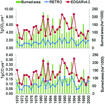
In the first part, past trends of CO2 and CO from fires were evaluated from two long-period inventories (data supplied by www.eccad.sedoo.fr), overlapping for the period 1970–2000. CO and CO2 were selected due to their role as greenhouse gasses, ingredients of smog chemistry, and their contribution on total carbon emitted by fires.
Then, we illustrated the differences and uncertainties in emission amount and spatial extend of emission estimates from five inventories at monthly basis, compared with the burned area pattern as recorded at provincial level by JRC.
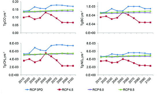
Finally, 21st century FEs for four species were illustrated, starting from the Representative Concentration Pathways (RCPs). The RCPs are a set of four new possible pathways of emissions and land use developments, based on consistent scenarios representative of existing literature (van Vuuren et al. 2011).
6.5.1 CO and CO2 Historical Trends
The basic characteristics of the biomass burning inventories used in this work are summarized in Table 6.2, and other information can be found at www.eccad.sedoo.fr.
The RETRO inventory (Shultz et al. 2008) is based on the analysis of available literature and datasets, estimates from different satellite products, and a semi-physical numerical model to simulate fire occurrence and spread. EDGAR4.2 (EC 2011) estimates FE from large scale biomass burning (savanna, grassland, and forest fires). It was developed on GFED2 inventory (van der Werf et al. 2006) for the period 1997–2005, while the data before 1997 were derived from GFED2 inventory scaled back with regional biomass burning trend from RETRO.
As for the temporal pattern, the two datasets seemed to well capture the inter-annual variability showed by the Italian burned areas (BA) from 1970 to 2000 (Fig. 6.2); peaks on FE estimations corresponded to peaks in burned area. For example, the RETRO maximum value (2.9 Tg CO2 and 0.18 Tg CO) was in 1990, when 1.95*105 hectares burned. Nonetheless, the extrapolation of a clear and reliable trend would be hardly possible. RETRO inventory showed a monotonic trend, characterized by a smooth inter-annual variability (range of 2.04 Tg CO2 and variation coefficient of 0.40 %), while the variability was more marked in EDGAR4.2 (range of 6.48 Tg CO2 and variation coefficient 0.37 %). The differences in CO estimations were smaller than CO2; in 1970 the difference was about 55 % against 73 % for CO and CO2, respectively. In 1990, the difference between the two products was still high for CO2 (66 %) and smaller for CO (44 %), while in 2000 it was about 56 and 23 %, respectively.
