Business Risk Measurement and Management in the Cargo Carrying Sector of the Shipping Industry – An Update
Chapter 25
Business Risk Measurement and Management in the Cargo Carrying Sector of the Shipping Industry — An Update
Manolis G. Kavussanos*
1. Introduction
Risk management in an industry which is riddled with cyclicalities in its rates and prices and which has made and destroyed millionaires over the years is extremely important. The issue has been discussed in Gray,1,2 comparing traditional methods of hedging, as he calls the choice of contract during ship operation,3 with the “new” instruments that appeared in the market at the time. The latter were the futures contracts, which were launched by the Baltic Exchange in London and the International Futures Exchange in Bermuda, trading BIFFEX (Baltic International Freight Futures Exchange) and INTEX contracts for the dry bulk and tanker sectors, respectively.
In the meantime a number of developments have occurred, including the restructuring, renaming and the eventual abandonment of the Baltic Freight Index (BFI) in 2002 – the underlying commodity upon which BIFFEX contracts have been trading. The development of Over the Counter (OTC) Freight Forward Agreements (FFA) since 1992, the introduction of clearing of these OTC contracts and the appearance of options and swaps can be added to these developments, all of which have major implications for the way risk is managed in the industry today. A comprehensive description of these developments is provided in Kavussanos and Visvikis.4,5
At the same time research has been published which has established formally a number of relationships not fully worked out previously empirically, and has uncovered new results on a number of important issues in the topic of risk measurement and management in the shipping industry. For instance, Kavussanos,6–10 measures for the first time the (time varying) volatility of ship prices and freight rates by sector and type of contract, thus allowing for a formal comparison of risk levels between sectors and freight contracts at each point in time. The later work by Kavussanos and Nomikos11–15 on the now-abandoned BIFFEX, of Kavussanos et al.16,17 and Kavussanos and Visvikiss (see endnotes 4–5)18,19 on FFAs and of Kavussanos and Dimitrakopoulos20 on Value at Risk (VaR) and extreme value methods has looked at significant issues underlying the freight derivative instruments and their use for risk management purposes. This chapter aims to provide a review of the issues in order to help the reader see where we currently stand.
Broadly speaking, the owner of the assets, ships, is faced with a number of commercial decisions. They include decisions on:
- Whether to enter the shipping industry by buying or leasing ships?
- What kind of ships to purchase?
- When to buy the ships and when to sell them?
- How to finance the purchase of the assets – debt, equity, shareholding, etc.
- Once owning the vessels, where to operate them and what kind of contract to seek for them?
- Whether to use financial instruments, such as futures and forward contracts, to manage the risk in such markets as the freight, bunker, foreign exchange and interest rate market?
These are all real decisions that the shipowner is faced with in everyday decision making. They all amount to viewing ships as investments – as assets in portfolios, which generate a stream of cash flows by operating the ships and a possible capital gain if selling the assets at prices higher than they are bought for. Given that commercial investments have risks attached, one can immediately see that the above issues are highly relevant for decision making. See Kavussanos and Visvikis (see endnote 4) for a detailed discussion of these.
The issues raised become more evident when examining the shipowner’s balance sheet, in Table 1. The shipowner’s cash flow problem is outlined in the table, where:
Cash Flow = Operating Revenue – Operating Costs (Fixed) – Voyage Costs (Variable) – Capital Costs (Fixed or Variable) + Capital Gain
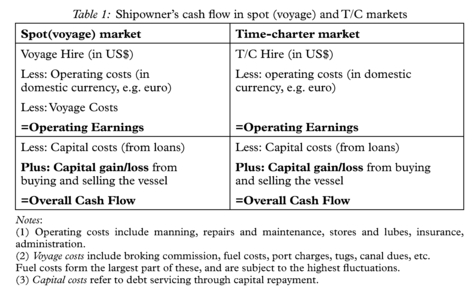
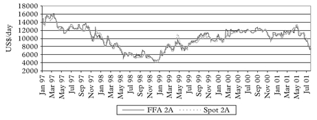
Fluctuations in revenue or costs can cause fluctuations in operating earnings. This may be due to changes in revenue, which is affected by changes in demand for freight services and by changes in freight rates, or because of changes in voyage or operating costs (e.g. changes in bunker prices, wage rates, exchange rates, etc). Operating costs include manning, repairs and maintenance, stores and lubes, insurance, administration, and are thought to be relatively constant, rising in line with inflation. In contrast to time charter markets, operations in the spot market involve voyage cost payments by the shipowner. Thus, apart from fluctuations in the freight market, owners are exposed to fluctuations in voyage costs, the main part of which are bunker prices. This is one of the reasons why spot markets are deemed riskier than time charter markets. The others relate to the nature of the relationship of spot and time charter rates, which leads us to expect that spot rates trade at a premium to time charters to compensate for the higher risk involved when operating the ships spot. The relationship is that, say, one-year time charter rates must be the sum of a series of expected (monthly) spot rates plus a risk premium. This is discussed fully in Kavussanos and Alizadeh.21
The volatility in freight rates, examined later in the chapter, and in Kavussanos (see endnotes 6–10), could be a source of risk. From the above table though it is apparent that voyage costs – in particular bunker prices – are the source of a certain volatility apparent when operating in the spot market, which does not affect the owner when operating in the time charter market. Alizadeh, Kavussanos and Menachof22 examine ways of mitigating bunker price risks through derivatives trading. They are discussed later in the chapter. Gray (see endnote 1) and Kavussanos and Visvikis (see endnote 4) discuss how selection of contract type can reduce freight risks, and Kavussanos (see endnotes 6–10) examines the same and other issues at the empirical level. The use of freight futures contracts (BIFFEX) for freight risk management has been examined in the past by Cullinane,23 Haralambides24,25 and Kavussanos and Nomikos (see endnotes 11–15). Finally, with the decline of interest in BIFFEX, Freight Forward Agreements (FFAs) and other financial instruments have provided the alternative for freight risk management. The issue is examined in Kavussanos and Visvikis (see endnotes 4,18) and in Kavussanos et al. (see endnotes 16,17). These are discussed later in the chapter.
The other source of risk for the owner apparent in the table is the interest rate risk. This relates to the capital charges, associated with debt finance. They fluctuate with interest rates. The higher the debt-equity ratio in the financing of a ship, the greater the financial leverage, and the more the residual cash flow is at risk. Thus, financial leverage compounds the risks created by operating leverage.
A further source of risk comes from the fluctuation in the value of the asset – the ship. Often, owners are involved in asset play, see Stopford26. They see ships as assets whose prices fluctuate, and offer the possibility of a capital gain or loss. This is shown in the last part of Table 1. Fluctuations in ship prices then influence the risk level involved in the investment. A major part of this chapter is concerned with this issue, which has been analysed in papers such as Kavussanos (see endnotes 6–10).
Credit risk, or counterparty risk, is yet another source of risk that shipowners face and it refers to the possibility that the counterparty in a private contract does not fulfil its obligations. This risk is more prevalent under bad market conditions and when the other party is losing money from the agreement. Such risk is prevalent, amongst others, in freight (voyage or time charter) contracts, in FFAs in bond issues, in interest swaps, etc.
In all the above, one has to add exchange rate risk, which is present in such an international industry. It affects the owner’s cash flow through a number of routes, including freight rates, voyage expenses, purchasing of the asset, etc. Interest rate and exchange rate risks fall outside the scope of this chapter. Sophisticated derivative instruments exist in the finance profession, which enable interested parties to deal with these risks – see Kavussanos and Visvikis (see endnote 4) for a description.
2. Risk/Return Trade-Offs in Shipping
In making commercial decisions the owner has in mind that greater rewards are usually achieved by undertaking higher risks. Usually such risks are measured by the volatility of the variable a decision has to be made for. For example, because freight rates fluctuate widely, say from month to month, taking a position in the market in a particular month can produce substantial gains or losses depending on what happens in subsequent months. Fluctuations in freight rates around their average values over a period of time may be used typically as measures of freight risk; technically, by their variance or by its square root, the standard deviation. High (low) standard deviations reflect high (low) volatility in rates and of the risks involved.27
Considering shipowners as asset holders, who wish to maximise return and minimise risk on their portfolio of shipping assets. Can they do anything to mitigate the risk involved in their shipping investments and in operations resulting from freight rate fluctuations? Say the shipowner is a specialist in the tanker sector. He is faced with two important decisions which can affect the risk/return position of his portfolio; (1) what size ships to invest-on? and (2) For a given investment, whether to operate the vessels in the spot or in the period (time charter) market? The issue of what size ships to invest-on, if approached from the pure asset-play point of view, may be answered by considering the risk-return profiles of different size vessels.
Vessel size considerations are important as the markets for each size are distinct in terms of the rewards and risks they carry, and so is positioning in the spot or time-charter market. From a different point of view, Glen28 has shown that the industry is divided into sub-markets. Kavussanos (see endnotes 6–10), shows that these markets are distinct in terms of their risk return profiles. As a result, investments in different size vessels can be thought of as having the same portfolio diversifying effects as different stocks included in an investor’s portfolio. To see that consider the possible disaggregation of the cargo carrying shipping industry discussed next.
3. Market Segmentation of the Shipping Industry
3.1 General cargo and bulk cargo movements
The parcel size distribution (PSD) of each commodity determines the shipping consignment of the cargo, see Stopford (see endnote 26). Some commodities are typically moved in larger sizes than others. For example, iron ore and grain consignments are much larger than phosphate rock or bauxite and alumna. Furthermore, the consignment size or PSD of each commodity changes over time and may be different on different routes. The PSD depends on: (1) Commodity demand and shipping supply economics (e.g. low value goods move in large consignments); (2) Transport distances (consignment is directly proportional to distance) and transport system restrictions (e.g. limited draft in ports, regulations); (3) Vessel availability. Consignments of over 2,000–3,000 tonnes can fill a whole ship (or hold) rather than part of a ship, and are typically transported in bulk. Smaller consignments, which fill only part of the ship (or hold), move as general cargo.
Bulk cargoes refer mainly to raw materials and are transported on a one -ship, one-cargo basis. They are further sub-divided into liquid cargo and dry cargo. Liquid cargo includes crude oil, oil products, chemicals (e.g. caustic soda), vegetable oils and wine. Dry Cargo is broadly divided in three categories: (a) Majors (i.e. iron ore, coal, grain, bauxite and phosphates), (b) Minors (i.e. steel, steel products, cement, sugar, gypsum, non ferrous metal ores, salt, sulphur, forest products, wood chips and chemicals; (c)Specialist bulk cargoes requiring specific handling or storage requirements such as heavy lift, cars, timber and refrigerated cargo. The ships involved in bulk cargo transportation are tankers, bulk carriers, combined carriers (they carry either dry or liquid bulk) and specialist bulk vessels. Bulk cargoes constitute two thirds of seaborne trade movements, and are carried mainly by tramp ships, which constitute three quarters of the world’s merchant fleet. These are vessels which move around the world seeking employment in any place/route of the globe. Bulk ships usually carry one cargo in one ship at rates negotiated individually for the service provided.
General cargo, is also dry cargo, but is not transported in bulk. A large part of general cargo is transported in containers, multipurpose and other specialised ships (Ro-Ro, car carriers, etc.). General cargo (one third of seaborne trade) is transported in either tramp ships or liners; the latter provide a regular, scheduled service, transporting small cargo consignments at fixed tariff levels between areas of the world.
The economics of each type of transport service are different. For example, oligopolistic conditions prevail in liner markets, while conditions of perfect competition guide tramp markets.
3.2 Bulk-cargo segmentation
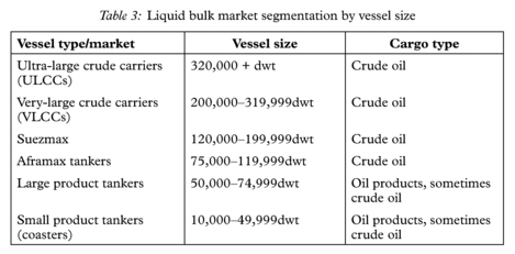
For analysis, dry and liquid bulk cargoes may be further subdivided according to the PSD functions of the products carried. The PSD function depends on the maximum size delivery an industry is able or willing to accept at any one time. In some industries stockpiles are around 10–15K tonnes, so a delivery of 50K tonnes is too large. Physical limitations on ship size draw a line between groups. For instance, Suezmax, Panamax, etc. This is because size determines the type of trade the ship will be involved in, in terms of type of cargo and route; this is a result of the different PSD’s of commodities and the port and seaway restrictions for certain size ships. Design features are important. For example, cargo handling gear (cranes), pumping capacity and segregation of cargo tanks in tankers; certain ports in developing countries cannot be used (e.g. ships which do not have cargo handling gear). Also, coating of tanks and ballast spaces are distinguishing factors. Tables 2 and 3 present the submarkets that are distinguished for dry and liquid bulk.
Very Large Ore Carriers (VROC) vessels (200,000+ dead-weight tonnes (dwt)) transport only iron ore from Brazil to West Europe (Rotterdam). They are VLCCs converted into dry-bulk carriers. Capesize vessels (100,000–199,999dwt) transport iron ore mainly from South America and Australia and coal from North America and Australia. Panamax vessels (around 60,000–99,999dwt) are used primarily to carry grains and
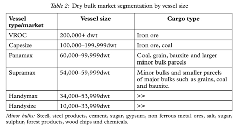
coal from North America and Australia. Handy vessels (around 10,000–59,999dwt) transport grains, mainly from North America, Argentina and Australia, and minor bulk products – such as sugar, fertilisers, steel and scrap, forest products, non-ferrous metals and salt – virtually from all over the world. Over time, in the category of Handy vessels, Handysize (10,000–33,999dwt) vessels have gradually become Handymax (34,000–53,999dwt), while Supramax (54,000–59,999dwt) vessels have appeared over the last years, as a consequence of vessel sizes becoming larger to satisfy the demand for larger PSDs for dry bulk commodities.
Smaller vessels such as Handy and Handymax in the dry bulk sector are, in general, geared so that they can load and unload cargo in ports without sophisticated handling facilities. They can avail of more ports compared to larger vessels. As ports
of the world have been developed the new generation of Handymax and Supramax vessels are carrying more and more of the trade the Handys carry. The same is also true in the liquid bulk sector; the very large vessels trade in only four-fifths of routes as the draught restrictions in ports and the storage facilities required ashore are very large to accommodate them and their cargoes. The smaller vessels are more flexible in terms of the routes and trades they are involved in. See Kavussanos and Visvikis (see endnote 4) for more details.
3.3 General (dry) cargo segmentation
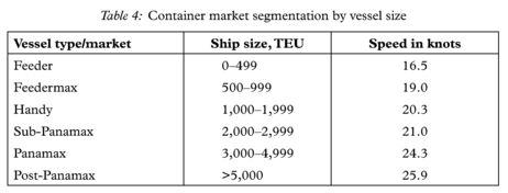
When general dry cargo is not moved by dry-bulk ships it is transported by liners. The following distinctions are common. Container ships, Ro-Ro, Multi Purpose MPP (Single-deck, multi-deck, Semi-containers), Barge Carrying vessels (BCV). Other specialised vessels include Refrigerated (Reefers), Car-carriers, Cement carriers, Heavy lift, Ore carriers, Vehicle carriers, LPG tankers, etc. Within the liner trades there is a move towards containerisation at the expense of non-unitised cargo which used to be transported in MPP ships. Containerships themselves have sub-markets according to size. These are shown in Table 4.
Just as with dry-bulk, each of these sub-markets has its own economic characteristics, and the risks and rewards involved for the shipowner and the charterers are different.
4. Comparison of Volatilities of Second Hand Ship Prices
Since smaller vessels can approach more ports (due to their smaller size and the existence of cargo handling gear on board) and can switch between different trades/routes they are more flexible for employment. As a consequence, they are less risky than the larger vessels. This is established in the market by the volatilities of both their prices and of their freight rates being lower than those of the larger vessels. This was first shown formally in Kavussanos (see endnotes 6–10), who compares freight rate and ship price volatilities between different vessel sizes. This is discussed next.
Having obtained data for freight rates and second-hand Handysize, Panamax and Capesize vessel prices, monthly returns and volatilities are calculated. These volatilities are compared between vessel sizes. Investments in vessels with higher volatilities are
Table 5: F-statistics for equality of unconditional variances in dry bulk ship prices
| Cape vs Panamax | Cape vs Handy | Panamax vs Handy | |
| F-statistic | 1.635 | 1.842 | 1.127 |
Notes:
(1) These statistics, which are defined as F=SD12/SD22~F(n-l, m-1), where SD12 and SD22 are the sample variances and follow the F distribution with (n-1, m-1) degrees of freedom; in this case (195,195) degrees of freedom.
(2) Critical values of the statistics at the 5% and 1% levels are 1.26 and 1.36 respectively.
(3) Sample period 1979: 5-1995:8.
Source: Kavussanos (see endnote 8)
Table 6: F-statistics for equality of unconditional variances in tanker ship prices
| VLCC vs Suezmax | VLCC vs Aframax | Suezmax vs Aframax | |
| F-statistic | 1.84 | 2.71 | 1.47 |
Notes:
(1) F distribution degrees of freedom (166,166), with critical values at the 5% and 1% levels 1.29 and 1.44, respectively.
(2) Sample period 1980: 2-1993:12.4.
Source: Kavussanos (see endnote 7)
deemed riskier compared to those with lower ones. Tables 5 and 6 show the results for the dry bulk and the tanker sectors, respectively.
Broadly speaking, for asset players who choose to have ships in their portfolio of assets they can reduce risk by investing in smaller vessels, compared to larger ones. Moreover, the results make sense as explained earlier. The smaller vessels are more flexible as assets. They have a lower risk of unemployment in adverse market conditions, as they can be switched more easily between routes and trades to secure employment. In addition, the cargo sizes that larger vessels carry makes them less useful for charterers requiring transportation of smaller quantities. This makes the demand for these vessels less flexible, and vessels cannot switch between sea-lanes and charterers as easily as their smaller counterparts. For instance, if anything happens (e.g. a political or economic change) in one of the routes the VLCC’s operate in this will have a significant impact in rates in the market, which is translated into high volatility in rates. As a consequence, the income stream from operations of smaller vessels, and their prices, as present values of the expected future income, are subject to less fluctuations in comparison to the larger vessels.
4.1 Dynamically adjusting volatilities
The studies by Kavussanos, (see endnotes 6, 7) mentioned above, have gone a step further in the analysis of ship price volatilities. They introduce, for the first time in shipping, the class of Generalised Autoregressive Conditional Heteroskedasticity (GARCH) models of Engle29 and Bolerslev,30 to estimate time varying volatilities of ship prices. Thus, price volatilities are explained in terms of their past values, values of squared shocks to long-run equilibrium in each market, and allow for the possibly of introducing a set of exogenous factors. The general form of the augmented GARCH-X(p,q) model of Bollerslev (see endnote 30) can be represented by the following equations:
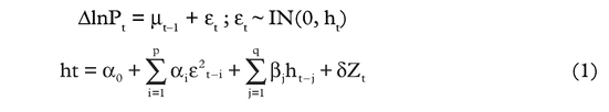

where, μt-1 is the specification of the conditional mean, that is, of the change in the log of ship prices, Δ1nPt, εt is a white noise error term with the usual classical properties and a time-varying variance ht, which may include a set of exogenous factors, Zt, and LL is the corresponding log-likelihood function after omitting the irrelevant constant. The parameters of interest are those included in μt-1, say φ(L), and the GARCH parameters α0,αi,βj and δ and can be estimated by maximum likelihood methods.
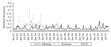
The estimated time varying volatilities allow the measurement and comparison of volatilities at each point in time, rather than relying on the averages over the period examined in Tables 5 and 6. Considering average volatilities(standard deviations) of ship prices (or freight rates) over a period of time as indicators of risk levels provides a partial picture of the risk/return situation. This is because uncertainty in prices, is not constant over time. The patterns and relative levels of volatilities, at each point in time (market situation) can now be measured, and compared between different ship sizes. Such estimates of time varying variances are also deemed important in the financial literature, as they may be used in the construction of dynamic portfolios of assets. These time varying volatilities of ship prices for the tanker and dry bulk sub-sectors are shown in Figures 1 and 2, respectively.
This method of analysing volatilities and examining them graphically has allowed further inferences for the dry bulk sector, such as that: Volatilities, and thus risks, vary over time and across sizes; in particular, volatilities are high during and just after periods of large imbalances and shocks to the industry. These include the period of the oil crisis of the early 1980s, the recovery period of 1986–1989 and the Gulf crisis of the early 1990s. Panamax volatilities are driven by old “news”, while new shocks
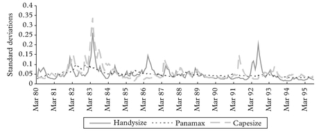
are more important in the Handy and Capesize markets. Also, conditional volatilities of Handysize and Panamax vessel prices are positively related to interest rates and Capesize volatilities to time-charter rates.
The three markets tend to respond together to external shocks, and yet quite differently, implying market segregation between different size ships. (i.e. there are some common driving forces of volatilities in different size markets, and yet there are idiosyncratic factors to each market that make each size-ship volatility move in its own way). These idiosyncratic factors relate to the type of trade each size ship is engaged in. Thus, volatility for Handysize and Capesize vessels has several hikes, while that for Panamax is smoother. This differing nature of volatil ities over ship sizes is manifested in the GARCH alpha(news) coefficients being higher than the beta (persistence) coefficients for Capesize and Handysize vessels, while the opposite is true for Panamax.31
Regarding volatility levels, Capesize volatility generally lies above the volatilities of the other two sizes, except for two–three years in the mid-1980s. Similarly, the Panamax volatility is, in general, at a level above Handysize, which, however, is exceeded at times by the hikes in the Handy volatility.
Similar results are reached by considering the time varying volatilities for the tanker sector. In addition, volatilities in the tanker sector and thus risks levels seem to be positively related to oil prices. The downward trends in volatilities observed in the dry bulk and tanker industry sub-sectors seem to indicate that risks in the shipping industry have decreased over time. It should also be mentioned that the availability of time varying volatility estimates for vessel prices, as with other assets in the financial literature, may be used as inputs in pricing derivative instruments such as options prices, etc.
5. Comparison of Volatilities of Spot and Time Charter Rates
Theoretically, ship prices are the present value of the expected stream of cash flows (profits) from their operation. The relationship has been investigated formally in
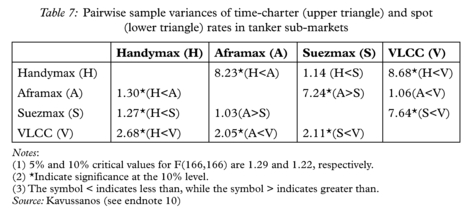
Kavussanos and Alizadeh.32 As a result of this theoretical relationship, comparison of freight rate volatilities by vessel size should reveal a similar relationship to that uncovered by examining the second hand prices. This is indeed the case; Kavussanos (see endnotes 6, 9) shows that volatilities of spot rates and of time charter rates are smaller for smaller size vessels, compared to those of larger ones. Table 7 compares these volatilities in the tanker sector.
In both the spot and time charter markets the VLCC sector exhibits the highest volatility compared to smaller sizes over the period examined. The Handymax volatilities are the lowest in both markets compared to other sizes. The Aframax and the Suezmax sectors show significantly larger volatilities in comparison to the Handymax sector and smaller ones compared to the VLCC in both the spot and the time-charter markets. However, the volatilities between the Aframax and Suezmax sectors are not statistically different between them. Overall, within the dry bulk and tanker sectors, risk levels, as expressed by freight rate volatilities, are different between vessel sizes. Coupled with the different levels of return each vessel size yields, different size vessels can be viewed as distinct asset classes in a portfolio of ships. This has implications for investors.
The above findings then, of the possible diversification effects that may be achieved by holding different size ships in a portfolio of assets have not been discussed in the literature previously. The studies by Kavussanos (see endnotes 4,7–11), have provided a formal justification of pursuing such strategies. In addition, these studies have also investigated, for the first time, empirically some well-known propositions regarding the possibility of operational risk reduction by choice of contract. Gray (see endnote 1) discusses the gradual risk reduction effects that are achieved by shipowners selecting to employ their vessels in markets such as voyage charter(spot), trip time charter, period time charter and in contracts of affreightment,33 consecutively.
Table 8 compares, statistically, pair-wise volatilities between the spot and the time-charter market for each size ship in the tanker sector. In all vessel sizes, but the Aframax, the spot rates are significantly more volatile compared to time-charters.