Biogenic Volatile Organic Compound Emissions
(3.1)
where n is the number of vegetation species emitting the jth isoprenoid,
 is the maximum seasonal value of basal emission from the T + L pool,
  is the maximum seasonal value of the basal emission from the T pool, ρnj is the biomass density of the n emitting species,
  and
and 
 are correction factors accounting for the gradient of light and temperature within the canopy due to sun shading,
  and
and  are the empirical coefficients of the Guenther algorithm for plants following a T + L emission mechanism (Guenther et al. 1995),
  is the empirical coefficient of the Guenther algorithm for plants emitting monoterpenes with a T mechanism,
  is the correction term accounting for the seasonal variations of the basal emissions.
In the model, different seasonality terms were adopted for deciduous and evergreen vegetation species. Values of ρnj in each grid cell were calculated by multiplying weekly values of the LAI, obtained from high resolved satellite observations (MODIS) performed in 2006, for the values of SLA of each one of the vegetation species present in the cell. SLA values were obtained by combining data from the literature with laboratory experiments. Values of on leaf temperature and incoming PAR radiation were collected from satellite observations and elaborated by partners of CarboItaly. Figure 3.1 highlights the high spatial resolution provided by the model, whereas Fig. 3.2 highlights its capability to provide isoprenoid-specific emissions. Both figures were obtained by integrating data elaborated on a 12 h basis. Such a distinction was important because many of the stronger monoterpene emitters followed a T + L mechanism.
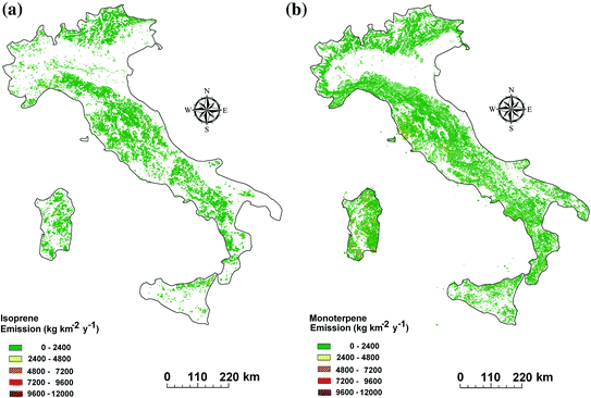
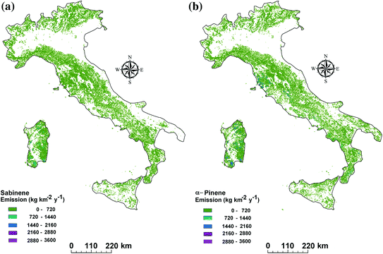
Fig. 3.1
Isoprene (a) and monoterpene (b) emissions for the year 2006 in Italy
Fig. 3.2
Annual emissions of sabinene (a) and of α-pinene (b) for the year 2006 in Italy
3.3 Results Provided by the Model and Validation
Data produced by our model confirmed the importance of monoterpene emission in Italy as their annual value (41.2 Gg y−1) exceeded that of isoprene (31.39 Gg y−1). More than 85 % of monoterpenes were found to be released from the T + L pool. About half of the emitted monoterpenes were composed by α-pinene (9.10 Gg y−1), sabinene (4.34 Gg y−1) and β-pinene (3.37 Gg y−1). Limonene, myrcene, trans– and cis-beta ocimene, linalool, 1-8 cineol, camphene, β-phellandrene and terpinolene contributed for the rest of the emission. Monthly maps showed that more than 70 % of the emission occurred between June and September, and it peaked in July. As shown in Fig. 3.3, seasonal trend predicted by our model for α-pinene released in the coastal site of Castelporziano for the year 2006 was consistent with flux measurements performed in 1997 (Ciccioli et al. 2003). Differences were mostly determined by the fact that the temperatures in August 1997 were much higher than those of the same month of the year 2006. As it can be seen, the contribution to monoterpene emission from deciduous and evergreen species following a T + L mechanism, produced a strong seasonal variation of the emission, with very small values in the cold seasons. Our model also indicates that the largest emission of isoprenoids occurs in Central-Southern Italy and the two Italian islands (Sardinia and Sicily). Isoprenoid emission is concentrated most along the Appennines mountain range separating the east from the west coasts of peninsular Italy. The intense light and temperature emission of sabinene in these areas, which has never been reported before, reflects well the dominance of F. sylvatica and C. sativa in forest ecosystems. The reduced emission of isoprene in these areas is instead determined by the fact that Quercus cerris L., which is one of the dominant species, is a very low isoprenoid emitter (0.1 µg leaf Dry Weight h−1). If confirmed by field measurements, these indications are of paramount importance in assessing the ozone production in the Italian peninsula as sabinene reacts much faster with OH radicals than α-pinene and it has a comparable reactivity with ozone.
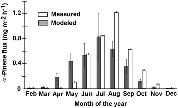
Fig. 3.3
Seasonal variations of α-pinene predicted by the model for the year 2006 in the coastal site of Castelporziano compared with fluxes measured in 1997
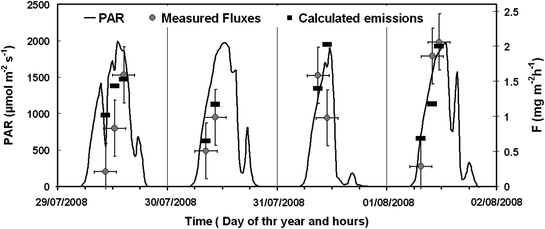
To confirm the importance of sabinene emission in the forest ecosystems located in the Apennines, a field campaign was held in a CarboItaly site largely dominated by F. sylvatica. The site (IT-Col) is located between 1,500 and 1,700 m a.s.l. between Forchetta Morrea, Prati S. Elia and Selva Piana, near the town of Collelongo (Abruzzo, Italy, see Sect. 2.2.8), at 95 km north-east from Rome. Around the measuring site and at that elevation (1,500–1,700 m a.s.l.) F. sylvatica is the dominant tree species for several hundred hectares. The BVOC sampling site, located in a clearing (Prati S. Elia, 700 m wide and 1,500 m long) was 1,000 m a part from the CarboItaly tower in operation since 1993 to measure the ecosystem exchange of water and CO2 by Eddy Covariance. By considering the complex shape of the area, the gradient method using tethered balloon profiles was the preferred approach to measure VOC fluxes. Only with this approach was indeed possible to collect samples above the average elevation of the canopy and to get values representative of a large area. By collecting VOC at 4 levels from 30 to 200 m above the clearing, sufficient data were available in order to get reliable values of the fluxes. They were measured from July 29th to August 1st 2008. VOC were enriched into cartridges packed with Tenax TA adsorbent resin using automated air sampling systems, equipped with temperature and pressure sensors to maintain a constant flow of air. Vertical profiles of temperature, pressure and relative humidity were also measured. After sampling, the cartridges were taken to the laboratory and analyzed within 10 days by a Gas Chromatography Mass Spectrometry (GC-MS) system equipped with a thermal desorption unit (Baraldi et al. 1999). Using the similarity approach, the Eq. 3.2 was used to calculate VOC fluxes (Kuhn et al. 2007