Ascertainment and Assessment of ES
and F. Müller10
(9)
Bundesamt für Naturschutz, Fachgebiet I 2.1 «Recht, Ökonomie und naturverträgliche regionale Entwicklung«,, Konstantinstr. 110, 53179 Bonn, Germany
(10)
Abteilung Ökosystemmanagement, Institut für Natur-und Ressourcenschutz, Olshausenstr. 75, 24118 Kiel, Germany
4.1.1 Introduction
The need for applications and tools of the–frequently mainly conceptually used–ecosystem service (ES) ideas has become more and more obvious during the last years (Daily et al. 2009). Practical applications are necessary to further develop and improve the conceptual base of ES on the one hand. On the other, tools for environmental and resource management are needed in order to further establish ES in decision-making processes (Kienast et al. 2009). The recognition and the appropriate quantification of ES are fundamentals for their valuation, independently whether the valuation is conducted with biophysical, social or economic methods. Their application and integration is one of the biggest challenges of contemporary ES science (Wallace 2007).
The supply of ES is based on geo-biophysical structures and processes, which are changing in intensity as well as in spatial and temporal distribution. Anthropogenic impacts, especially land-use and land-cover changes or climatic variations are among the major factors determining the qualities and quantities of ES supply. Land-use patterns and changes in land cover can be surveyed, spatially analysed and regionally assessed. They deliver direct measures for human activities (Riitters et al. 2000) and clearly demonstrate the relations between ES supply and demand (Burkhard et al. 2012). Spatially explicit identification and mapping of ES distributions and the analysis of their spatio-temporal dynamics therefore enable the aggregation of highly complex information. The respective ES visualisations can support decision-makers in the environmental sector by providing powerful tools to support sustainable landscape planning and ES trade-off assessments (Swetnam et al. 2010). Spatially explicit ES quantification and mapping have therefore been named as one of the key requirements for the implementation of the ES concept in environmental institutions and decision-making processes (Daily and Matson 2008).
One key problem of each ES quantification is, besides the difficult and comprehensive data acquisition, the selection of an ES categorisation system which is appropriate for the specific study region and the particular research question. Most of the currently available ES classification systems (e.g. de Groot et al. 2010a; Wallace 2007) distinguish the three classes with regulating ES, provisioning ES and cultural ES. Some authors additionally include habitat services (de Groot et al. 2010a; TEEB 2010). Habitat services are, however, often assigned to the category of ecosystem functions, which in the Millennium Ecosystem Assessment (MEA 2005a) were called supporting ecosystem services. Many ecosystem functions or habitat properties do not deliver direct or final ES. Therefore, the distinction between ecosystem functions and ES has become more common and accepted. This distinction also proved to be advantageous for the avoidance of double counting of closely correlating functions and services, for example in monetary valuations.
Numerous methods and tools for the characterisation of ecosystem functions and services in landscapes have been developed especially within the last 10 years. Additionally, existing methods and data collection programmes are ready to be integrated in the ES concept due to their thematic diversity (e.g. monitoring within the long-term ecological research (LTER) network; Müller et al. 2010). They include measurements, monitoring programmes, mapping activities, expert interviews, statistical analyses, model applications or transfer-functions (de Groot et al. 2010b). Natural structures and processes (e.g. flows of energy, matter and water) are central in biophysical assessments. These approaches are different from monetary valuations, where the actual assessment of values is carried out by monetisation. Monetary ES approaches such as cost-benefit analyses (CBA) or willingness-to-pay (WTP) surveys are applicable and well-established concepts (Farber et al. 2002). However, results are often disappointing especially for nonmarket goods and services such as many regulating ES, ecosystem functions or biodiversity characteristics (Ludwig 2000; Spangenberg and Settele 2010).
Suitable ES indicators are needed for all quantification approaches. These indicators have to be quantifiable, sensitive for land-use changes, temporally and spatially explicit and scalable (van Oudenhoven et al. 2012). Indicators are tools for communication, enabling the reduction of information about highly complex human-environmental systems. After Wiggering and Müller (2004), indicators in general are variables delivering aggregated information about certain phenomena. They are selected to support specific management purposes by providing integrating synoptic values, depicting not directly accessible qualities, quantities, states or interactions (Dale and Beyeler 2001; Turnhout et al. 2007; Niemeijer and de Groot 2008).
4.1.2 Ecosystem Service Supply and Demand Assessment at the Landscape Scale–the ‘Matrix’
Different landscapes can be characterised by different ecosystem structures, functions and consequently by varying capacities to supply ES (Burkhard et al. 2009), depending on the natural settings as well as human activities (e.g. land use) within the research area. Different land-use patterns, heterogeneous population distributions as well as multiple ecological and socio-economic conditions cause varying demands for ES (▶ Fig. 3.2).
In this chapter, a method for the assessment of different land-cover types’ capacities to support ecosystem functions (assessed based on the ecological integrity concept and respective indicators for ecosystem structures and processes; for detailed information see Müller 2005; Burkhard et al. 2009, 2012), to supply multiple ES and to identify demands for ES will be shortly introduced. The method has been applied in different case studies, for example for the assessment of ES in boreal forest landscapes in northern Finland (Vihervaara et al. 2010), in urban–rural regions in central eastern Germany (Kroll et al. 2012) or for the calculation of flood regulation capacities in a Bulgarian mountainous region (Nedkov and Burkhard 2012).
The approach is based on an assessment matrix, which links relative and mainly non-monetary ES supply capacities or ES demand intensities to different geospatial units (e.g. different land-cover types). Based on this interrelation analysis, resulting ecosystem function and ES scores can be visualised in maps. Differentiations between ES supply and demand but also between ES potential and de facto flows (ES actually used by humans) are needed (see below). Supply and demand of/for different ecosystem goods and services are often spatially and temporally decoupled and managed by transport, trade and storage opportunities in today’s globalised world. Nevertheless, calculations of these two variables deliver data that are highly relevant for ES budget assessments for specific spatial or temporal units. Self-sufficiency rates and ES flows within and between regions can be calculated on this basis. Ecosystem functions and several regulating ES such as nutrient regulation, erosion control and natural hazard protection are exceptions. They are normally not transportable and therefore, a physical connection between the service providing unit (SPU) and service benefiting/demand area (SBA) must exist (Nedkov and Burkhard 2012; Syrbe and Walz 2012; ▶ Sect. 3.3).
Such information, especially in a regionalised form, and the related ecological and socio-economic data are highly relevant for environmental management and for ES-based landscape planning. Thus, requests for appropriate tools are numerous (Kienast et al. 2009). When assessing the potential of a landscape, a land-use type or an ecosystem, usually the (hypothetical) maximum of ES supply under the given conditions is being assessed. Often it is not considered whether there is a human use of these ES or not. Flows of ES on the contrary describe the capacity of a defined spatial unit to supply a specific ES set (ES bundle) actually used by humans within a given time period (after Burkhard et al. 2012; see Box). This distinction becomes relevant for certain ES, for example when assessing protected ecosystems. These systems undoubtedly supply numerous goods and services. However, e.g. in the case of core zones in national parks, where any human activity may be prohibited, many of these ES (e.g. timber, game) cannot be used. Of course, ecosystem functions, such as nutrient cycling or biodiversity, take place anyway. They provide positive effects on ecological integrity within the protected area itself, but often also on adjacent ecosystems. For many regulating ES, it can be assumed that ES potentials and flows are comparable (▶ Sect. 2.1).
4.1.2.1 Conceptual Background for ES Supply and Demand (after Burkhard et al. 2012)
ES supply refers to the capacity of a particular area to provide a specific bundle of ecosystem goods and services within a given time period. For detailed analyses, a differentiation between ES potentials and actual ES flows is needed.
ES demand is the sum of all ecosystem goods and services currently consumed or used in a particular area over a given time period. Up to now, demands are assessed not considering where ecosystem services actually are provided. These detailed provision patterns are part of the
ES footprint which (closely related to the ecological footprint concept; Rees 1992) calculates the area needed to generate particular ecosystem goods and services demanded by humans in a certain area and a certain time. Different aspects of ecosystem service generation are considered (production capacities, waste absorption, etc.) for assessing the ES footprint.
Ecosystem functions, ES supply, ES demand and ES budgets in different land-use types can be assessed by the help of ES matrices. The first matrix in ◉ Fig. 4.1 contains ecosystem functions (ecological integrity) and ES on the x-axis. The geospatial units (here CORINE land-cover types; EEA 1994) are placed on the y-axis (after Burkhard et al. 2009, 2012). All relevant ES capacity scores are entered, using a relative scale between 0 (equivalent to no relevant capacity to support the respective ecosystem function or to supply the respective ES), 1 (low relevant capacity), 2 (relevant capacity), 3 (medium relevant capacity), 4 (high relevant capacity) and 5 (maximum capacity in the study area) at the intersections. Based on the 44 different CORINE land-cover classes and 39 ecosystem functions and services, altogether 1716 capacity scores have to be given (◉ Fig. 4.1). Due to this high number of scores needed and the related high assessment efforts, existing databases or expert evaluations need to be harnessed. These data can successively be checked and replaced by more exact information resulting from modelling, measurement, monitoring or in-depth interviews (Burkhard et al. 2009).
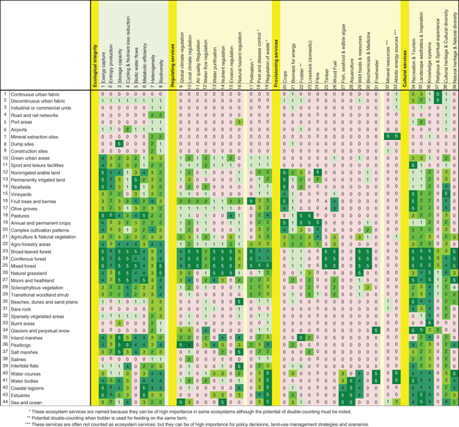
Fig. 4.1
Land-cover types (y-axis) and ecosystem functions and services (x-axis) illustrating the capacities of different land-cover types to support ecosystem functions and to supply ES on a scale from 0 (no relevant capacity; pink) to 5 (maximum relevant capacity; dark green); exemplarily assessed for a central European ‘normal landscape’ (after Burkhard et al. 2009, 2012)
The matrix in ◉ Fig. 4.1 shows clear patterns of ES capacity distributions across the different land-cover types. Especially, the forest land-cover types (including broad-leaved, coniferous and mixed forests) show high scores for a multitude of ES. Such multifunctionality is typical for forest ecosystems. Also the other generally more natural land-cover types such as natural grasslands, wetlands and water bodies are characterised by high ES capacities. Strongly anthropogenically influenced ecosystems, such as urban fabrics, industrial or commercial units and transport units (in the upper part of the matrix), show comparably low ES capacities. Of course, these areas also supply ES, but in comparison with the other land-cover types, their ES supply is rather low (▶ Sect. 6.4).
The whole ES concept is a highly anthropocentric approach. Fisher et al. (2009) defined that only those services with a clear benefit to human societies can be denoted as ES. Services without direct human benefits should be termed as ecosystem functions or intermediate services. Thus, a societal demand should be identifiable for all individual ES. Data about actual anthropogenic uses of each ES are needed for their assessment (see definitions in Box 1). Major parts of this information can be derived from statistics, modelling, ecological and socio-economic monitoring or from interviews. ◉ Figure 4.2 shows a respective matrix, which, comparable to the ES supply matrix (◉ Fig. 4.1), provides exemplary information about the ES demands within the different CORINE land-cover classes. The y-axis contains regulating, provisioning and cultural ES. The ecological integrity variables are not relevant here because they (per definition) do not provide direct benefits to humans. The scores were given in a similar manner as in the ES supply matrix; 0 (light pink) denotes no relevant human demand within the particular land-cover type and 5 (dark red) illustrates maximum demand.
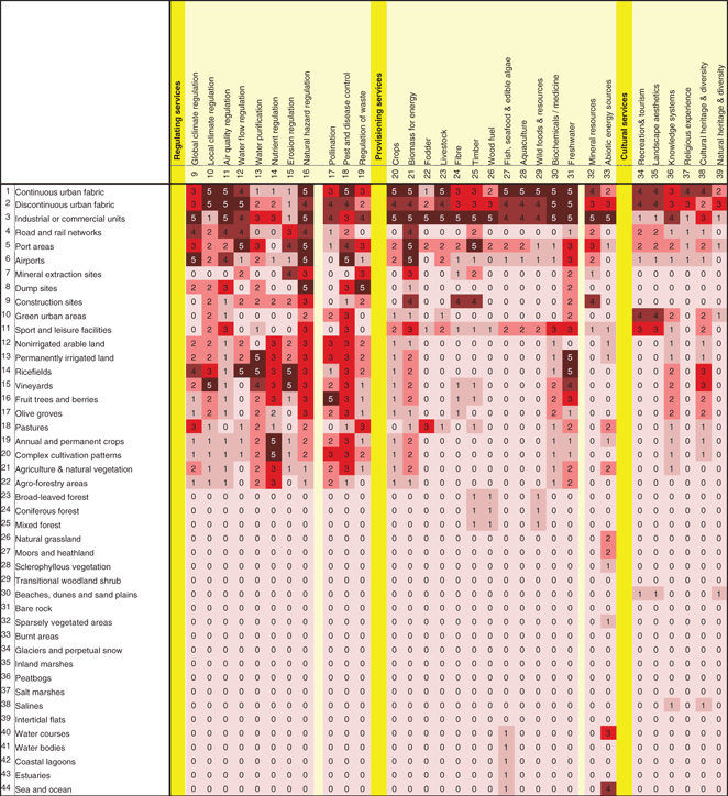
Fig. 4.2
Demand for ecosystem services (x-axis) within different land-cover types (y-axis) on a scale from 0 (no relevant demand; light pink) to 5 (maximum demand; dark red); exemplarily assessed for a central European ‘normal landscape’ (after Burkhard et al. 2012)
◉ Figure 4.2 clearly shows that the overall highest demands for manifold ES are located within the highly human-modified land-cover types in the upper part of the matrix. Urban areas as well as industrial and commercial areas are the land-cover types with the highest demand scores. It also becomes obvious that in the more natural land-cover types (lower part of the matrix), generally lower demands for ES can be found. This can of course be justified by the lower population numbers and related lower consumption rates in these areas. Agrarian land-cover types show high demands for regulating ES (e.g. nutrient regulation, water purification, erosion control). Similarly to the ES supply matrix, ES demand maps can also be compiled based on the ES demand matrix.
Taking the information from the ES supply and demand matrices as starting points, sources and sinks for individual ES can be identified. As both components–supply and demand–were normalised to the same relative units (0–5), ES budgets can be calculated by subtracting the ES demand scores from the ES supply scores. And also the resulting ES budget scores can be illustrated in a matrix and in maps. ◉ Figure 4.3 shows the ES budget matrix for the different CORINE land-cover types. Each field in the ES budget matrix was calculated based on the scores in the ES supply matrix (◉ Fig. 4.1) and the ES demand matrix (◉ Fig. 4.2). Therefore, the assessment scale ranges from −5 = demand clearly exceeds supply (undersupply), via 0 = demand = supply (neutral budget), to + 5 = supply clearly exceeds demand (oversupply). Empty fields indicate land-cover types with neither a relevant ES supply nor a relevant demand for ES.
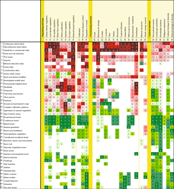
Fig. 4.3
Ecosystem service supply-demand matrix showing budgets in the different land-cover types; based on matrices in Figs. 4.1 and 4.2. Scale from − 5 (dark red) = demand clearly exceeds supply = undersupply; via 0 (pink) = demand = supply = neutral budget; to 5 (dark green) = supply clearly exceeds demand = oversupply. Empty fields indicate land cover types with neither a relevant ES supply nor a relevant demand for ES (after Burkhard et al. 2012)
◉ Figure 4.3 shows a clear pattern of ES undersupply in the regions with high anthropogenic influences, especially in the urbanised areas and the industrial and commercial units. The more natural land-cover types, particularly the forests, show characteristic patterns where the ES supply often exceeds the demand. More detailed information about the locations of actual ES supply (SPUs) and related flows to areas of ES demand (SBAs) could be integrated in ecosystem service footprint calculations (see Box 1). No experience with this approach is available up to now. Highly complex import and export balances would be needed, for which data on required scales are not easily available.
The following case study application from the central eastern German region Leipzig-Halle shows how empirical ES quantifications can be transferred to the relative 0–5 scale, and how the results can be illustrated in spatially explicit ES maps. The study took place as a part of the EU project PLUREL (Peri-urban Land Use Relationships, ► www.plurel.net/). More detailed information about the different ES quantification methods and the map compilation can be found in Kroll et al. (2012) and in Burkhard et al. (2009, 2012). The following maps from the Leipzig-Halle case study region include CORINE land-cover maps for the years 1990 and 2006 and spatial distributions of the provisioning ES ‘energy’ supply, demand and supply–demand budgets (◉ Figs. 4.4 and 4.5). The quantifications for the ES ‘energy’ refer to final energy units in gigajoule per hectare per year. Lignite as the major energy source in this region was included within the provisioning ES category. We are aware that current ecosystem functions are not involved in the generation of lignite and that the integration of natural resources is seen critical by many authors. We are following the CICES system (► http://cices.eu/) here, which includes abiotic outputs from natural systems in their accompanying ES classification. Moreover, open-pit lignite mining has enormous impacts on ecosystem structures and processes in the study area’s landscapes. Thus, this ES is of high relevance for landscape planning and therefore cannot be neglected.
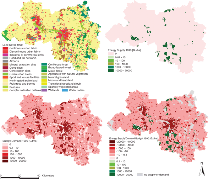
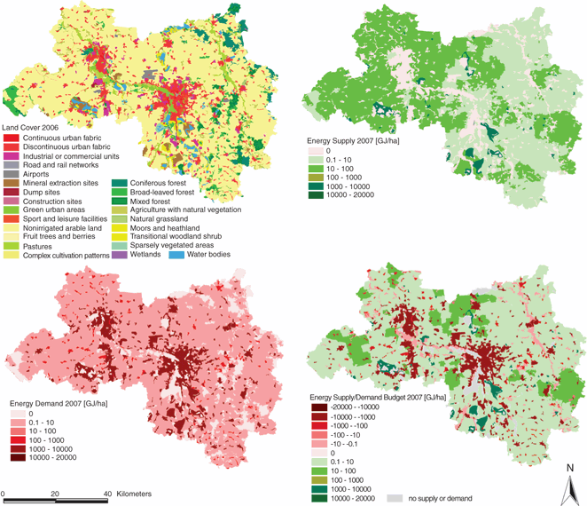
Fig. 4.5
CORINE land-cover map 2006 (top left); energy supply map (top right), energy demand map (bottom left) and energy budget map (bottom right) for the Leipzig-Halle region in the year 2007 (energy data in GJ ha−1 a−1; after Burkhard et al. 2012)
The energy supply map from the year 1990 (◉ Fig. 4.4, top right) shows that the large lignite open-pit mines were the only regional energy source at this time with a final energy contribution of 20,000 GJ ha−1 year−1. In the year 2007 (◉ Fig. 4.5, top right), a clear reduction of the open-pit mine areas and their energetic outputs are visible. New energy sources such as wind power, biomass, solar energy or waterpower were developed, resulting in a more heterogeneous distribution of energy supply in the region.
The demands for the energy provisioning ES (◉ Figs. 4.4 and 4.5, bottom left) show a clear sink function of the industrial and commercial units and the urban areas. The pit mines themselves also have a high demand for energy. The demand for energy was generally decreasing by 20 % between 1990 and 2007, mainly due to the decline of energy-intensive industrial activities and energy saving measures. The ES supply–demand budget maps (◉ Figs. 4.4 and 4.5, bottom right) illustrate the abovementioned source-sink functions of the rural and urban areas. Based on such information and data, decisions for regional ES provision and landscape planning can be supported.
4.1.3 Conclusions and Outlook
The high applicability of the ES matrix approach presented here arises from its potential for visualisation and from the comparison of the effects of different land-use activities on ecosystem functions and services. Thereby, assessments of trade-offs between different land-use types are possible. Various ecosystem functions and services can be displayed and huge amounts of data resulting for example from expert interviews, statistics, measurements and modelling can be integrated. The normalisation to the standardised relative 0–5 scale integrates different biophysical dimensions (e.g. Joule, tons, diversity indices) or economic units (e.g. Euro, Yuan) and makes them (to a certain degree) comparable.
The application of freely available spatial data such as CORINE enables the coverage of large landscape units with a unified land-cover classification system in almost all European countries. Issues with the land-cover classification system, the spatial data resolution and generalisation problems lead to uncertainties of the assessments. Further data with higher spatio-temporal or thematic resolution can, like in the ES assessments, easily be integrated.
The matrix approach is also linked with technical and thematic uncertainties, especially if the majority of the ES scores are based on expert opinions. The uncertainties are based upon the selection of a suitable and representative case study area, the selection of relevant land-cover classes (matrix y-axis), spatial and geo-biophysical data acquisition, the selection of relevant ecosystem functions and services (matrix x-axis) and related indicators, the indicator quantification in the matrices based on the 0–5 scale, the linkage of the assessment values with the spatial units (map compilation) and the interpretation of the results by the end user. A detailed discussion of the different sources of uncertainties can be found in Hou et al. (2013).
Further developmental steps are needed to tackle these problems. One key issue is the inclusion of additional ES in the quantitative classifications, as shown in the energy budget case study example. Direct measurements, official statistics, simulation models or specific surveys, for example in the class of cultural ES, are needed to fill these data gaps. Moroever, regional geological, geomorphological, pedological, climatic and geobotanical site conditions as well as additional human system inputs (e.g. fertiliser, energy, materials) strongly influence ES potentials and flows. These effects should be integrated in future assessments (besides land-cover and land-use intensity) in order to minimise the assessments’ uncertainties. Thereby, more exact ES scores (0–5) can be provided for example to actors in participatory processes.
Nevertheless, there are limits of intersubjectivity in such an optimisation. Related to the high amount of data needed to derive the different ES matrices, it will probably not be possible to completely abdicate from expert opinions. This statement can of course be interpreted as a critical argument. But it can also be seen positively because expert-based approaches have the advantage of relatively rapidly delivering target-oriented results which immediately can be applicable in decision-making processes.
One major demand from environmental planning is to make predictions about potential future developments’ effects. Therefore, one key step in the future improvement of the matrix approach is the coupling with computer models (▶ Sect. 4.4.3). This would enable assessments of scenarios and their spatial specifications regarding the supply and demand of ES. This would seriously increase the applicability of the ES concept in practice. Due to the enormous complexity of such efforts, only common, transdisciplinary and cross-regional efforts will lead to positive outcomes.
4.2 Approaches to the Economic Valuation of Natural Assets
B. Schweppe-Kraft11 and K. Grunewald12
(11)
Bundesamt für Naturschutz, Fachgebiet I 2.1 «Recht, Ökonomie und naturverträgliche regionale Entwicklung«,, Konstantinstr. 110, 53179 Bonn, Germany
(12)
Zöllmener Str. 11 b, 01705 Freital, Germany
4.2.1 Principles of Economic Valuation
“It is not with money that things are really purchased. (John Stuart Mill 1848)”
Economic science is, briefly put, the art of the rational and economical use of scarce resources for the fulfillment of human values and needs. Since ecosystem services are limited and their use is often at least partially mutually exclusive (trade-offs), rules are needed to make rational choices between alternatives that affect ES more or less strongly. Here, economic science seeks to maximise the general welfare, taking into account intergenerational welfare, distribution and consensual ethical rules.
Ecosystem services become economic goods, or obtain economic value, by providing benefits, and by being scarce. Not only such goods as food, water and recreational opportunities provide benefits; so, too, do the nonmaterial assets that are part of human preference and thus relevant as benefits. The right of species to exist and the value we ascribe to that right are–besides other more direct benefits–of economic importance, as soon as they become a part of individual preference. Thus, the habitat function of an ecosystem for wild species may constitute a sociocultural ES in this sense.
Scarcity means that the provision or maintenance of an ES is associated with costs (Baumgärtner 2002). An example are the costs of measures to maintain ‘healthy’ landscapes that provide sufficient opportunities for recreation, fertile soils, fresh water, etc. (▶ details in Sect. 6.5). Almost 50 % of the biological diversity in Germany relies on traditional or nonintensive forms of land use that are usually not economically competitive on the world market. The resources for conserving such anthropogenic biotopes and habitats are scarce. Costs can arise even if no money is paid, for example from the limitation of agricultural and forestry use in protected areas. These so-called opportunity costs are, generally speaking, benefits which the society or the individual must do without, in favour of other goals or benefits.
Ecosystems continually provide people with services. They are similar in this respect to the human-made productive assets that are used to provide us with goods and commodities. Such assets are the basis of our welfare, unless they are consumed or destroyed. The same holds true for natural assets as well: ‘We must live from the interest, and should not consume [natural capital]’ (Hampicke and Wätzold 2009). Destroyed or degraded ecosystems are restorable, if at all, only after a long period of time. The costs of restoration generally exceed the cost of maintenance many times over. The genetic information lost by species extinction is irreversible. Nonetheless, the economic value of the depreciation of natural capital is not easy to determine.
Unlike buildings, industrial plants or machinery, natural capital usually provides us with a number of different benefits simultaneously, each of which has to be evaluated separately. These generally include so-called public goods, such as air quality regulation, recreation in the open countryside, etc. One of the characteristics of public goods is that they cannot be privately appropriated. Therefore, there are no functioning markets which could lead to an optimum level of supply based on individual supply and demand. Market prices can be interpreted as values in the sense of willingness-to-pay and as costs, expressing scarcity. All this is lacking in the absence of markets.
In addition, each single ecosystem is embedded in a tight network of ecological dependencies with other natural assets. In such a situation, the assessment of physical changes can already be a problem, long before we arrive at the point of valuation. Moreover, there are also creeping impacts which occur later, and when they occur, then sometimes in an erratic and irreversible way. Which means, that methods, like the discounting method, are required to compare current and future costs and the difficult problem of valuing nonmarginal changes has to be solved.
If economists valuate goods or services, they as a rule assign them instrumental value, based on their usefulness for achieving a defined objective. This means that both economic valuation and the ES concept approach the issue from an anthropocentric perspective (Hampicke 1991). In addition, economic valuation is based on ‘methodological subjectivism’ (Baumgärtner 2002). All valuations must (or at least should, see below) build on the preferences of each individual citizen.
Economic assessments are always focused on choices between alternatives. Ecosystem services, like any other goods and services assessed in an economic cost-benefit-analysis, are not evaluated in isolation, but always in terms of their relative advantage in comparison with other goods, which, due resource scarcity, must be dispensed with. The relative advantage of one asset compared with others is its economic valuation, which, for practical reasons, is not expressed in terms of specific goods (e.g. ‘How many glasses of beer is something worth to me?’), but rather in terms of the maximum amount of income which one will forego, or the maximum willingness-to-pay/ minimum willingness-to-accept, of individuals. All methods of economic evaluation, including the market-based and cost-based methods, try in principle to value (real) income changes and willingness-to-pay more or less accurately, or at least to find plausible proxies for such valuations.
Economic valuation, must, in accordance with its own principles and methodological standards, always focus on specific alternatives, e.g. restoration or no restoration of an alluvial floodplain; maintaining a grassland or converting it into farmland; urban living conditions with or without an adjacent park, etc. Economic valuations of ES are often part of a so-called cost-benefit analysis, which attempts, as far as possible, to evaluate all the economic impacts of the implementation and of the nonimplementation of a project or programme, or of various project or programme alternatives. To this end, all relevant effects of the various alternatives must first be predicted. As regards public goods, such as recreation, urban living conditions or urban climate, this encompasses an assessment of the number of persons who will benefit or suffer disadvantages due to a change with respect to these goods. Moreover, all costs, savings, income increases and income declines must be determined, including all costs and benefits measured in income equivalents (willingness to pay or to accept) which will result from the changes in public goods.
The final step in a cost-benefit analysis, as in any economic evaluation, is the aggregation of individual values to a total value. This is done by adding all positive and negative income effects (costs and benefits) including the observed income equivalents (willingness to pay). This means that, for example, the social value of the preservation of the recreational function of a landscape and of the habitat function of its ecosystems for flora and fauna is nothing but the sum of individual willingnesses to forego income in favour of the maintenance of these functions. The social value of a land development project, e.g. an industrial plant, would result from the net income growth caused by the new plant, minus the willingness to pay for the lost recreation and conservation functions, minus the agricultural land rent (which is usually included in the price paid for the land by the new owner), minus all other external costs not included in the price, such as increased flood damage or flood regulation costs caused by the additional water run-off due to imperviousness of the land surface.
The process of evaluation and aggregation is somewhat similar to an election (Osborne and Turner 2007), but with some differences:
The individual can only vote in accordance with the scope of his own interests (How often does he really use a recreational area? What is the share of the income generated that accrues to him?).
The strength of a vote can differ (a greater or lesser increase in individual incomes or of income equivalents measured by willingness-to-pay).
The individual is not directly asked to vote; rather, his ‘vote’ is ascertained from the extent (positive or negative) of the net income effect accruing to him.
The net income effect does not have to be investigated for each person individually, it is sufficient if the sum is known.
Representative sampling methods are applied to determine the benefits of public goods (▶ Sect. 4.2.3).
Economic valuation methods differ from the ‘one man, one vote’ rule, inasmuch as every individual valuation of public goods is in fact tied to the amount of individual earnings, i.e. valuation results can depend on income distribution. Normally, it is not the purpose of a cost-benefit analysis to examine the fairness of distribution. In industrialised countries, this is no problem, for income distribution is as a rule irrelevant to the results of a cost-benefit analysis. Different weightings for individual willingness to pay in order to compensate for income disparities usually affect the overall results only slightly. This may be different if the effects of an international scope are assessed. Ignoring income inequalities on an international scale can easily result in ethically unacceptable valuation approaches.
The abovementioned principles of economic valuation:
Are based on individual preferences
Assess values as relative advantages, expressed in terms of changes in income or income equivalents (willingness-to-pay)
Involve the formation of a social value by simple aggregation of individual values
They do not mean that economic valuation completely denies the notion of values that are not simply individual, but which rather have supra-individual worth, such as divine commandments, animal rights, or the notion of binding rules for a harmonious human-nature relationship. Cost-benefit analysis accepts such values, but treats them as individual ones, assuming that they are solely valid for the person that proclaims them. A person who assumes, for example, that animal rights should be ranked higher than the pursuit of any additional welfare gains, cannot demand that all economic advantages measured in a cost-benefit analysis be set to zero. He can, however, demand that his own individual foreseeable future income growth be assessed as his willingness-to-pay against e.g. any further species extinction.
Accordingly, individuals and their choices based on individual preferences tied to their economic limits (income) on the one hand constitute elementary declarative units. That means that the economic value is determined by the subjective evaluation of individuals ascertained by means of a survey of representative samples. In the strict sense, expert judgments can only be integrated into cost-benefit analyses if they can be interpreted as approximations to the preferences of individuals which cannot be measured directly. In this view, the economic value assigned to an ES is not a quality that is inherent to that object (e.g. an ecosystem), but rather a value which depends on the overall context, not only the economic context.
The valuation of the ES ‘fresh drinking water’, can, for example, depend on the following aspects (Baumgärtner 2002): How much clean water is there in total? How is the supply of clean drinking water distributed in space and time? How is the access to this resource regulated? What competing demands for water exist, besides its use in households? What kind of institutional restrictions exist? What kind of alternatives are there to water use in various use areas, and what would they cost? How much would it cost to import clean water from other regions? How much does technical water purification cost?
The failure of the market, private production and private consumption to generate socially-acceptable or optimal results–i.e. a market failure–is, according to economic doctrine, the occasion for an economic evaluation. This may be the case if:
Production and consumption cause losses of benefits or price increases for others (so-called negative external effects). Examples: intensifying agriculture by removing hedgerows impairs the recreational capacity of a landscape; diking along a river can prevent flooding of areas behind the dike, but increases the flood risk upstream and downstream.
Public goods are involved, i.e. those which benefit a large number of people without or with only limited possibilities of excluding anyone from those benefits. Example: recreational use of the open landscape, of public bathing waters, the existence value of species/biodiversity, or possible future pharmaceutical use of a certain kinds of species. In such cases, due to the lack of user payment, there are no incentives for market activities to maintain the provision, to prevent overexploitation, or to protect the asset from detrimental external effects.
The costs of current activities accrue over the long term, e.g. to future generations, and therefore are not taken into account by present market participants. For example soil erosion, CO2 emissions by intensive agricultural use of peat soils.
In the case of market failure, economic valuation has the function of informing about all costs and benefits accruing to people now and in the future, and enables decision-makers to reduce external costs and maintain provisioning with public goods to an optimal extent, thus maximising welfare under consideration of all relevant costs and benefits.
Like public surveys and public participation, cost-benefit analysis can help ascertain public opinion more precisely and make individual preferences more obvious than can be done by general elections only. In addition, it can reveal a malfunction of the democratic system, for example, the lopsided influence of powerful interest groups which are able to effect political decisions against the public interest (e.g. environmentally counter-productive subsidies; Brown et al. 1993).
Economic valuations need not necessarily be carried out with monetary units (Abeel 2010). Money can even be a hindrance. It can, for instance, promote the idea that only the world of market goods (production and consumption) really counts, whereas the actual goal is to correct the results of the market, by making it clear that the production of goods entails hidden costs that can obscure their true prices. Often, we are persuaded to produce things that we would rather do without for other, nontraded goods, e.g. for biodiversity and healthy ecosystems, if we knew enough about the issues, or if it became obvious that national income consists to a considerable degree of the costs of repair of damage to the environment and nature (Leipert 1989).
Money as a valuation unit may moreover suggest that the valuated goods will in fact be priced and thereafter traded. Nonetheless, the decision as to how to deal with market failure is up to policy makers, and is completely independent of the valuation process. Whether market failure is to be corrected by public supply, by do’s and don’ts, by incentives, by taxes, duties or user fees or by the creation of markets, is a matter for public decision making. Economic valuation does not imply converting public goods into commodities to be traded on the market, either directly or indirectly.
Another misconception may be that the value of an ES that is calculated and determined for a specific social, economic or ecological environment could be transferred to other situations with no adaption, like the price of a good trade on the world market, for instance a smart phone. Such an understanding, however, would overlook the fact that many ecosystem services are tied to their point of origin, so that no distribution can take place. However, distribution in response to demand is a prerequisite for the emergence of a common price level on the market.
On the other hand, valuation in monetary terms can be highly practical. A monetary value allows a trade-off involving costs, income and various other goods, including public goods, based on the views of a representative sample of citizens. Other valuation methods, such as benefits analysis (Zangemeister 1971; Hanke et al. 1981) and similar types of so-called multi-criteria analysis (Zimmermann and Gutsche 1991), also use decision-making models based on trade-offs (▶ Sect 4.1.). However, such models often depend on the opinions of a limited selection of experts and/or ‘citizen experts’ (Dienel 2002), which are not representatives. Although in certain cases, expert-based models may have a high problem-solving competence, the social values upon which they often implicitly build have not been validated.
Various decision-support instruments, such as cost-benefit-analyses, expert-based multi-criteria analyses or discursive processes of active citizenship, should be used in accordance with their respective strengths and weaknesses. A representative group of citizens mixed with some experts could for instance provide useful advice for the best use of a fixed local budget for various urban green-space management measures; however, when it comes to the preparation of a concept for reducing soil erosion in a district (Grunewald and Naumann 2012), an expert-based cost-effectiveness analysis would likely be better grounds for sound decision-making. The cost-benefit analysis, after all, shows its strengths when actions are to be taken that might affect a great number of people physically and financially in very different ways. This is the case, for instance, when decision support is needed on the question as to how much money a city should spend overall on green-space management. Another example would be the design of a well-balanced programme of measures for reducing soil erosion that should also take into account other effects, e.g. upon species preservation, the landscape, or water pollution, in such a way that the costs of the measures will best be outweighed by their benefits.
Example
Grossmann et al. (2010) applied a cost-benefit analysis on proposals for a bundle of nature-based flood prevention measures by increasing the retention area through dyke-shiftings (▶ Sect. 6.6.3). They calculated the avoidance of flood damage, valuated the water purification effect of an enlarged alluvial floodplain by comparing it with the cost of alternative measures for reducing water pollution, and asked people about their willingness-to-pay for the benefit of the enhancement of conservation and recreation. The value of the ES thus assessed was three times as high as the cost of the measures.
4.2.2 The Total Economic Value
The most widely accepted approach for the economic valuation of ES is the concept of Total Economic Value (TEV, Pearce and Turner 1990) (◉ Fig. 4.6). The various benefits of ecosystems are classified as either use values or nonuse values. Use values are further subdivided into direct and indirect use values and option values. Nonuse values are broken down into existence values and bequest values.
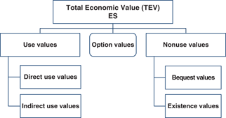
Direct Use Values
Direct use values accrue from the direct use of ES for consumption and production, e.g. food, firewood, medicine, timber, drinking water, cooling water, etc. The use of a landscape for recreation, leisure activities, tourism or scientific or educational purposes is also considered a direct use of ES (Baumgärtner 2002). Direct use can be consumptive–example: firewood–or nonconsumptive, as with recreation. Direct use values are linked to provisioning services and goods, as well as with some sociocultural ES, such as for recreation, cultural identity, landscape aesthetics and knowledge services.
Indirect Use Values
Indirect use values arise when ecosystem services interact directly or indirectly with human activities. Examples are flood control by means of water-retention measures in alluvial floodplains, the self-purification effect of water bodies, or the water-filtration capacity of soils. The so-called regulatory services generally fall into this category. The economic value of these services is measured as the change in the costs and benefits of the use that is affected by them, e.g. reduction of flood damage, benefits from additional use as a swimming location, or the decreased costs of the drinking water supply; see, by analogy, the concept of final ecosystem services by Boyd and Banzhaf (2007) (▶ Sect. 3.2).
Option Values
Option values express the fact that there is a willingness to preserve the possibility of later use of ES, regardless of whether this will really take place or not. Option values and values to be realised in the future correspond largely to the so-called Potentialansatz (capacity approach) in German landscape planning (▶ Chap. 2 and ▶ Sect. 3.1). The option value can also be interpreted as an insurance premium that people are willing to pay to maintain the possibility of future use (Weitzman 2000). Option values are especially significant in the context of landscapes and ecosystems of high cultural significance and singularity, such as the Brocken peak in the Harz Mountains in Germany, or with respect to the uncertainty of a future economic use of species and their genomes (e.g. Norton 1988).
Bequest Values
The bequest value expresses the willingness of people to forego parts of their present income in order to preserve things for future generations. This heritage can refer to sociocultural ES, but also to provisioning services.
Existence Values
Existence value reflects the willingness-to-pay for the preservation of things regardless of whether there is any likelihood of their future use or not, just in order to preserve their existence. Such values are often ascribed to assets thought to have an intrinsic value, such as living species, e.g. in the concept of animal rights.
These different kinds of values, named above, are conclusive. Their sum is the overall economic value of an ecosystem. However, in field studies, it is often impossible to clearly separate the different values from one another.
Investigations at Natura 2000 sites have revealed that more than 50 % of their TEV were constituted by indirect use values and nonuse values (Jacobs 2004). That means that from a conservationist point of view, these values, especially the option, bequest and existence values, are the most critical ones. On the other hand, the problems of reliable evaluation increase as one moves from direct use values to nonuse values.
4.2.3 Valuation Methods and Techniques
4.2.3.1 Use Values
Market Prices
If assets provided directly by nature can also be found on markets in the same or a similar quality–e.g. mushrooms, fish, game–the market price can be used as a proxy for their value (the market-price method). One important precondition for the applicability of this method is that product qualities and the demand for marketed and non-marketed products are similar. This is not always the case, however. For example, experience shows that blueberries which are picked in the woods on a hike taste particularly good, this special kind of appropriation seems to give them an extraordinary quality, so that they could be rated considerably higher than purchased blueberries. On the other hand, the picking is an activity that is incidentally performed, without significant additional effort. One might also pick the berries when demand is low, and therefore have to valuate them at a price well below their market price. The same is true of self-caught fish. As an actively appropriated product, it might have a higher value than comparable market products, but it could also serve as an incidental by-product of the fishing activity itself, which is the actual ES provided–recreational activity. If the fish is used by the family of the angler, their possibly differing preference for fish may also be important for the valuation.
The market-price method could, for example, be suitable for the valuation of the effect of an alteration in forest management on all the wild fruits to be found there, or it could be appropriate for the valuation of the improved water quality in a lake on the composition of its fish population (less biomass, but a higher proportion of game fish). In both cases, the changes on the supply side are only one side of the coin, for the extent to which the additional supply will really be used must also be assessed. Finally, the question should be answered, e.g. on the basis of surveys, to what extent the value of the products is thought to lie above or below the market price level.
Change of Value Added, Profits, Return on Sales Minus Cost of Production
The majority of market goods created with the help of ecosystem services, such as drinking water, wood products, food, etc., is produced in combination with labour and capital. If the ES change, e.g. additional land used for agricultural production, causes increased sales of goods, the additional value of sales is not the only determining factor for their valuation; rather, it is the difference between the additional sales and the costs of the use of capital, precursor products, production facilities and labour power, including a normal remuneration of the labour input of the entrepreneur. The difference remaining after this calculation corresponds in the case of e.g. cropland more or less to the cost for the lease of the land being assessed, or a comparable plot. Therefore, the ground rent (lease) is often used as a proxy for the net value of the productive input of ecosystem services that are combined with certain plots of land (Hampicke et al. 1991).
Example
What loss in the value of agricultural production would result from the abandonment of this field (◉ Fig. 4.7)? From the total loss of market revenue, one must first subtract the variable costs. In addition, adjustments with respect to labour and capital inputs will occur in the mid- or long-term and have to be considered in the evaluation. After these adjustments, the loss of ground rent (lease) remains as a permanent loss. This is determined on the basis of various favourable and unfavourable factors, such as soil fertility, water supply, climate, slope, etc. When evaluating large-scale soil loss in developing countries, one would have to assume significantly higher income losses, due to a lack of alternative employment opportunities. Nothing in the world would suffice to persuade us to do without the entirety of the agricultural land on earth–its loss would have a value of ‘minus infinity’ (Costanza et al. 1998).
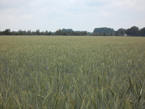
Fig. 4.7
The economic value of the provisioning service of a field (here cornfield near Sulingen in Lower Saxony) can be measured on the basis of the income loss resulting from abandoned agricultural use. © Burkhard Schweppe-Kraft
If a corn (maize) field is converted into a species-rich damp meadow, for example due to conservation measures, a comparison of these two different provisioning services–corn and hay, respectively–would require a calculation of the difference between the proceeds from the sales of these two products, and of the above-described production costs. For the corn, this difference would be positive; for the hay, probably neutral or even negative.
For a comparison of the total economic value (TEV) of intensive–e.g. corn–and extensive farming systems–e.g. a meadow–a correct valuation of the services corn and hay could be critical. The difference between the profits is often significantly less than the difference between the sales proceeds, one reason being that intensive farming systems often require higher inputs. The different valuation of provisioning services, in one case on the basis of sales proceeds, in the other on the basis of sales proceeds minus costs, explains why in the study by Ryffel and Grêt-Regamey (2010), the calculated total value of species-rich grassland is less than that of intensively used grassland, while in the study by Matzdorf et al. (2010), the species-rich grassland comparatively outperforms the farmland (▶ Sect. 6.2.4).
An assessment of provisioning services on the basis of sales proceeds would mean that not only ES would be evaluated, but the value added by labour and capital, too, would be included. A correct application of the cost-benefit analysis must always subtract the costs necessary for production from the value created, to calculate the net yield. In the case of provisioning services, this means the respective earnings minus the wages for the work of the contractor plus the rent paid for the land (see environmental services ▶ Sect. 2.1).
Implicitly, the above calculation of provisioning services involving profits or rents is based on the assumption that the labour thus ‘freed’ and–at least in the medium to long term, even the capital thus ‘freed’–will find uses elsewhere, and will there generate added value that corresponds to the costs. Cost-benefit analyses carried out in industrialised countries are, due to the flexibility of the markets for labour and capital, generally based on this simplifying assumption. Deviations should be clearly identified and explained. In many regions in developing countries, however, the necessary alternative opportunities are not available, particularly for the factor labour. If the destruction of the services of an ecosystem, e.g. the loss of soil fertility, or overfishing, drives the people who had depended on these services into long-term unemployed, the cost-benefit analysis would have to include as the value of the supply service concerned not only the lost profits, but the entire value, including labour and possibly capital costs. In industrialised countries like Germany, adjustment problems and deadlines are more likely to be the factors to be taken into account with respect to the factor capital.
Therefore, when determining the cost of a change in agricultural production or the abandonment of agricultural use the calculations for the short or medium term are often based on contribution margins. A contribution margin is the market revenue minus the variable costs. As the term implies, the contribution margin per hectare states the contribution that the production on one hectare of land makes to cover the fixed costs of a business, for example, to the interest payments due on the loan for stables (see case study in ▶ Sect. 6.2.3). A contribution-margin calculation assumes that unused capital is inflexible, i.e. it cannot be used elsewhere just as profitably. In the short term, such a method of calculation is justified; in the medium term however, adaptation possibilities have to be assumed. After the technical depreciation period of the capital involved–at the latest–it is advisable to shift to such values as lease or long-term profit outlook for the calculation of production losses. The correct handling of the costs of capital can be crucial for the actual calculated results. For example, in a case of the rewetting and use abandonment of previously farmed peat soils, Röder and Grützmacher (2012) calculated costs of € 40/t of saved CO2 emissions, on the basis of contribution margins. If only the lease costs of, say, € 250/ha were used in the calculation, a much more favourable value of around € 9/t of CO2 would result. Assuming a 20-year adjustment period with adaptation rates at a consistent level and a calculated interest rate of 3 %, costs of over € 17/t would result. Calculation examples from studies based on all three types of calculations can be found in the literature. This shows that major methodological differences occur not only in the evaluation of ES generally, but also that great tension is possible simply with the very conventional cost calculations, which are based on different, and often highly questionable, assumptions.
The example of using land-lease as an approximation for the long-term value of the agricultural production function of an ecosystem (provisioning services) again shows dramatically that economic valuations generally apply only to relatively small changes: The higher total value of grassland compared to farmland, which can be calculated on the basis of the study by Matzdorf et al. (2010) (▶ Sect. 6.2.4), applies only to the case of the current distribution between grassland and farmland. If, due to the currently high total economic value (TEV) of grassland, ever more farmland were to be transformed into meadowland, the supply of the various public and private goods produced using these land areas would gradually increase so greatly that the prices and the willingness-to-pay for any additional margins of these goods would fall. The total economic value per unit of converted farmland could pull even with the TEV per additional unit of grassland, and then even exceed it. This could in fact be accomplished relatively quickly, for example in the case of the species-protection function/service. For the preservation of biodiversity often optimally requires a mix of grassland and farmland, and not a grassland monoculture.
This also shows why the value of the sum of all ES cannot be calculated from the value to be set for a relatively small change to be assessed. Multiplying the total stock of farmland in the industrialised countries by the respective lease values per hectare, the result is by no means the value that society would be willing to pay for the preservation of the agricultural production output of these areas; the true figures would be significantly higher. With the increasing loss of production areas, prices would rise to an extreme degree, and the social upheaval thus provoked would have uncontrollable consequences.
Example
Within the EU, the service pollination is estimated at a value of some € 14 billion (Gallai et al. 2009). This is the value of agricultural products which are highly dependent on insect pollination. This knowledge does not help much for concrete valuations. In assessing the changes in pollinator populations in specific growing regions, the decisive factor is whether the populations there already constitute a limiting factor for production, or whether they are extant in abundance. So far for example, we know relatively little about how flower strips within fruit-growing areas impact on the net yields (◉ Fig. 4.8).
Fig. 4.8
Fruit growing areas are particularly dependent on pollination services. © Burkhard Schweppe-Kraft
Change in Production Costs
The cost of production method also ascertains the change in the difference between the sales proceeds and costs of production, but it does so for the special case that product quantities and revenues remain constant, and that only the costs of production change. The typical example of this case is the reduced effort required to provide clean drinking water if a farm field, which generates pollution is replaced by grassland. Another example would be an increased use of fertilisers to compensate for reduced soil fertility, which has resulted, for example, from intensive use, or soil erosion caused by the removal of hedgerows and other small structures.
In these cases, the production cost method was used directly to valuate the supply capacity of ecosystems (water supply, agricultural production), and also indirectly to assess the impact of regulatory services (reduction of soil pollution, and of soil erosion by small structures) upon the respective provisioning service.
Damage Costs, Mitigation Costs, Adjustment, Repair, Replacement Costs
Many regulating services influence the effects of natural hazards (flooding, avalanches and mudflows, storm damage, etc.) and anthropogenically induced risks (climate change, air pollution, urban climate stress). For the evaluation, the damage and damage prevention costs and the adaptation, repair, replacement or avoidance cost can often be used. Here, the extent to which damages (including medical expenses), or the cost of prevention and repair (rehabilitation) can be changed by ecosystems and ES is examined. Examples include the prevention of flood damage through restoration of floodplains, or avoidance costs for the treatment of respiratory diseases caused by the dust-filtration effect of urban green spaces.
It is a general economic principle that a goal should be achieved at minimum cost. If a damaged item is of lower value than the cost of its repair, it is more beneficial to all concerned to monetarily compensate the aggrieved person than have the damage repaired. This principle applies not only to the compensation for damage to passenger cars, but also to evaluation in the determination of total economic value (TEV). The same applies if the damage-avoidance costs are higher than the damage. Here, too, it is cheaper to pay the lower insurance compensation for a damaged asset than the higher cost of completely avoiding the potential cause of damage. Such situations are referred to as the least-cost principle.
Often, only a portion of the value of an ecosystem services can be quantified by damage or repair costs, just as medical costs often reflect only the cost of treatment, but not the physical or mental suffering of the patient. If, due to increased use intensification in an area, there are no more skylarks or partridges there, the cost of resettlement or avoidance of that loss may be significantly less than its ethical and aesthetic significance. Other methods, such as willingness-to-pay analyses, should be used if damage or avoidance costs can measure only part of the total economic value of a service.
Example
During the mid-1990s, Pimentel et al. (1995) assessed the on-site and off-site costs of erosion in the USA, and arrived at a figure of about $100/ha/yr. If this order of magnitude of replacement and damage costs is compared with the cost of erosion-mitigation measures, a very positive cost-benefit ratio of 1:5 results; the soil erosion hazards due to water and wind are thus reduced from 17 t/ha−1 a −1 to 1 t/ha−1 a−1. Using an analogous approach for a loess-covered, predominately agricultural area in Saxony, Grunewald and Naumann (2012) ascertained a cost-benefit ratio of approximately 1:2 (▶ Sect. 6.6.2).
Alternative Costs
Closely connected with the above methods is the so-called alternative-cost approach. This method often valuates not the costs in fact incurred, but rather those of theoretically possible options which might be used in order to achieve a goal in an alternative manner. An example might be the evaluation of the additional self-cleaning capacity of a renaturated water body, using the two potential alternatives of, on the one hand, the measures necessary to reduce pollutant input from agriculture, and on the other, the building of additional wastewater treatment capacity to achieve the same water-quality effect. The erosion protection provided by hedgerows and small structures could, for example, be valuated not only via the production-cost method, as above, but also on the basis of the cost of soil conservation measures on the field which are equally effective.
Whether or not a corresponding alternative-cost approach is permissible depends on whether the social goals are formulated in a sufficiently binding manner or not. Strictly speaking, the alternative-cost approach only leads to correct results if the objectives are formulated in such a binding manner that the necessary measures for their alternate achievement will actually be implemented in the not-too-distant future. An example of such a binding social goal is the EU Water Framework Directive (WFD), which mandates the attainment of a certain level of water quality (▶ Sects. 3.3.2 and 6.6.2). If farmland is converted to grassland, the nutrient input into the groundwater and the surface waters is reduced, and the specified goals of the WFD become more attainable. A corresponding contribution to the reduced water pollution can be achieved by various measures in farming, or by improvements in the treatment stages. Under the least-cost principle, an alternative measure, which allows both similar relief at the lowest cost and at the same time has a realistic chance of implementation should be selected as the value of reduction of nutrient immissions due to conversion into grassland. Matzdorf et al. (2010) used a value of between € 40/ha and € 120/ha for the valuation of the reduced nutrient inputs through the preservation of grassland, based on the evaluation of data of cost-effective measures to reduce nitrogen emissions by Osterburg et al. (2007) (▶ Sect. 6.2.4).
Measures for rewetting and restoring formerly farmed peat soils halt the mineralisation of organic soil components, and thus lead to a significant reduction of greenhouse-gas emissions. The evaluation of this regulatory service ‘rewetted peat soils’ is possible both on the basis of damage costs and on the basis of alternative cost. In accordance with the Stern Report, the methodological convention of the German Federal Environment Agency (UBA 2007) suggests a preliminary cost estimate of approximately € 70/t of CO2, based on a combined damage-/mitigation-cost analysis. In case of the use of wind power, 1 t of avoided CO2 emissions costs approximately € 40; on the European carbon market, a ton of CO2 cost € 6–7 in early April 2012. Which of the above values is to be used for the valuation of the CO2 emissions saved by rewetting will depend on how future developments are to be assessed (▶ Sect. 6.6.4).
It can be assumed that the required reduction of CO2 emissions cannot be implemented solely using the current favourable measures that enable the current low prices on the carbon market. Achieving the goal at these costs is thus unrealistic. Measures in the cost category of CO2 avoidance through wind power would seem, for example, to be more realistic. If we assume, moreover, that the goal of limiting the temperature increase to 2°C will fail to be attained by a wide margin, which seems increasingly likely, even the € 70 damage costs would have to be considered too low. The example shows that even with realistic assumptions, there can be very widely divergent evaluation approaches. Evaluations should therefore always disclose the assumptions upon which they are based, and whenever possible, alternative calculations under different assumptions should be undertaken.
Example
At the beginning of the 1990s, the city of New York was forced to take action, since it no longer met the established drinking-water quality standards. A water filtration and treatment plant was to be built for $ 6–8 million, and operating costs of about $ 300 million per year would have been added. As an alternative, the issue of improving the ecological functions of ecosystems in the Catskill Mountains, the drinking-water catchment area for the city, was examined. This cost was estimated at a one-time investment of € 1–1.5 billion. Faced with a balancing of interests between the cost of improving the ecosystems on the one hand and the development of purification technology as a substitute for the reduced ES of degraded ecosystems on the other, the decision was made in favour of the ES option (Chichilnisky and Heal 1998).
Real Estate Prices–Hedonic Pricing
The evaluation approaches presented above have, under the MEA (2005a) system and the ES classification (▶ Sect. 3.2), respectively, been oriented primarily towards provisioning and regulating services. The hedonic pricing method is oriented towards the sociocultural services recreation and aesthetics, or beyond that and in more general terms, towards the subjectively evaluated welfare functions of green elements and green spaces in the residential environment.
Under the hedonic pricing method, the goal is to ascertain the effect of near-residential green spaces on real-estate prices by statistical analysis. Hoffmann and Gruehn (2010) come to the conclusion that in densely populated inner-city districts, the green features of the residential environment accounts for 36 % of the property value. In less densely populated, smaller towns, the effect is less (▶ Sect. 6.4).
The hedonic pricing method covers only that portion of the use of urban green spaces that accrues indirectly to the property owners. Any benefits above this portion would have to be ascertained by other methods, by carrying out an additional willingness-to-pay analysis, or on the basis of the statistical data estimates of a demand function, similarly to a travel-cost analysis.
The Travel-Cost Approach
The term travel-cost analysis covers a whole package of different methodological options, which are primarily used for the evaluation of recreation areas. Here, the relationships between the number of trips to a region or a certain type of area and the amount of the cost per trip are analysed statistically. In the newer versions of the method–also the quality of the area for recreation (e.g. landscape, landscape diversity, facilities with recreational infrastrucure) are taken into account. On this basis, a demand function for recreation in the area or area type in question is assessed. Based on a comparison of the behaviour of visitors with high- and low-access costs, respectively, it is possible to deduce that the willingness-to-pay for the first visit undertaken within a given monitoring period to a particular area or type of area is higher than for later visits. Visitors with low access costs do not need to exercise this higher willingness-to-pay for the first visit in real terms, and thus realise a so-called consumer surplus. The sum of all consumer surpluses yields the total net benefits of recreation in the assessed areas. The consumer surplus constitutes the willingness-to-pay that an individual has for a recreational activity, minus its actual cost.
In some proposed methods and evaluation studies (Ewers and Schulz 1982; UBA 2007; to some extent too, Getzner et al. 2011), the actual costs of a recreational activity are regarded as its benefits. Certainly, assuming rational behaviour, the benefits must generally be at least as high as the cost paid for them; however, as discussed above in connection with the costs for the production of agricultural products, the purpose of a cost-benefit analysis is to ascertain the difference, or the ratio of costs to benefits, for each alternative. With such a difference ascertainment, the result of a recreational activity the benefits of which are just as high as the costs, would always be neutral; the net benefit, i.e. the difference between benefits and costs, would always be zero. This result would emerge in all studied alternatives, regardless of whether the recreation areas were of average quality, are actually upgraded, or would be devalued by impacts. For it we dispense with the counterbalancing of the costs, and show the cost only in their indicator function for the minimum benefit, we will arrive at completely nonsensical evaluation results when comparing options. For example, if the construction of a bypass road were to lead to an increase in the expense of money or travel-time to be paid by the inhabitants for access to their recreation areas, this would not be recorded as an obstacle to their recreation, but rather as an increase in their recreational benefits. Hence, the simple calculation of cost is unsuitable for the evaluation of recreational benefits. The goal must be to calculate the consumer surplus, the difference between the benefits (or willingness-to-pay) and the costs.
Under the travel-cost method, which uses this approach, willingness-to-pay is derived from the observed actual behaviour of a large number of different recreation-seekers, using statistical methods. This, like the land-price method, is one of the so-called revealed-preference methods, based on an investigation of factually evident preferences, in contrast to the stated-preference methods, in which the preferences are directly queried.
Example
In the Eibenstock-Carlsfeld region in the western Ore Mountains of Saxony, a survey was carried out via interviews among visitors and tourist-service providers on their appreciation of the landscape scenery (Grunewald et al. 2012). The questions concerned the qualitative landscape characteristics and preferences, travel expenses and willingness-to-pay for the maintenance and appearance of the landscape. For this purpose, the monetisation approaches of the travel-cost and willingness-to-pay methods were used. The study comprised face-to-face interviews with 95 summer and 105 winter tourists; travel costs were recorded for a total of 584 individuals. The goal was the analysis and monetary valuation of sociocultural ecosystem services related to landscape aesthetics, in order to provide a foundation for the improved landscape planning and management.
The tourists’ aesthetic perception of the landscape elements in the region is influenced primarily by visible, near-natural landscape elements, such as the forest and water bodies, and by their harmonic composition. An undisturbed landscape was the principal reason for travelling to the region and spending vacations there. Altogether, tourists paid about € 5.5 million per year in travel costs (extrapolated to the total number of tourists visiting the region), they are willing to pay € 170,000 per year in addition for the protection and management of ecosystems. The results show that the visitors valued public goods and services highly, a factor which will have to be considered more strongly in future planning (Grunewald et al. 2012).
Hunting Leases, Fishing Licences, etc.
For some recreational activities, such as hunting or fishing, there are prices to be paid in the form of fishing licences and hunting leases. These, unlike such expenses as those for fishing equipment or the fuel used to reach a fishing spot, are an expense associated with no real costs, or only minimal ones. A payment that is not remuneration for any labour or capital cost is referred to as a ‘surplus.’ Even the rent for agricultural land is such a ‘surplus.’ By paying for a hunting lease or fishing licence, the sportsman shows that his benefit from the fishing or hunting activity is at least equal in value to that payment. In this case, as with the land-price method, this share of the benefits accrues not to him, the user, but rather to the owners of the land leased. The benefits that can be calculated from fishing or hunting leases is the lower limit of the actual benefits from that activity.
If we also wish to ascertain the net benefits to the anglers and hunters over and above this minimum, it would be necessary to apply other methods, such as the travel-cost approach or contingent valuation. It is important in cases of changes in the conditions for recreational use, to always also ascertain the possibilities of substitution. Generally, there are also other places where recreational activities may be carried out. In such cases, the increase in travel costs to remaining alternative fishing or hunting areas would be a first rough measure for the welfare loss caused by the degradation or the loss of another area. With a more precise travel-cost analysis, it would be possible to capture also the ‘consumer surplus’ over and above simple cost effects.
Admission Prices
A method for calculating leisure and recreational use which was in the past particularly common is the admission-price method. Here, the recreational opportunity to be valuated–from city parks to national parks–is compared with similar recreational activities for which a price of admission is charged. One problem with this method is that people who spend time in fee-based recreational facilities, such as former horticultural exhibitions or amusement parks, may have different preferences from those of people who use free leisure facilities, such as urban forests or natural parks, so that it is difficult to find truly comparable situations. For example, admission-charging swimming pools and guarded beaches often have a distinctly different character than free swimming spots. Moreover, the price of admission reflects the lowest level of willingness-to-pay among those who avail themselves of the service; some visitors would be willing to pay a higher ticket price. Because of these problems, a valuation based on admission prices should also be supplemented by some other alternative valuation method, such as travel-cost or willingness-to-pay analysis.
The Willingness-to-Pay Analysis (Contingent Valuation), Choice Analysis
In addition to, or as an alternative to the above methods, any direct or indirect use value can theoretically be assessed on the basis of direct interviews using contingent valuation or the choice analysis. These valuation techniques are used for the ascertainment of both use and nonuse values (see below). Applied to the same evaluation object, travel-cost and willingness-to-pay analyses often provide relatively similar results (Löwenstein 1994; Luttmann and Schroeder 1995; Whitehead et al. 1995). In cases where specialised knowledge is required for an evaluation, e.g. for the evaluation of changes in soil fertility, erosion, effects on water quality, flood damage, etc., complementary expert-based methods should also be used, in addition to the willingness-to-pay analysis, in which, since it is a representative approach, largely nonexperts are interviewed.
4.2.3.2 Methods for the Detection of Nonuse Values
Contingent Valuation, Choice Analysis
Preferences for nonuse values, such as the desire to preserve species and habitats as a ‘value in and of itself’ (existence value), or so that they can be used and experienced by future generations (bequest value), can, like option values, currently only be ascertained by direct, representative surveys. The main methods for this are the willingness-to-pay analysis and the choice analysis.
The willingness-to-pay analysis asks how much money or income an individual would be willing to do without, as a maximum, in the form of a generally mandatory landscape-maintenance tax, so that nature might be preserved, or a specific conservation programme might be implemented. In a choice analysis, the respondents are presented with different options about the future, which they can, by means of various procedures, either accept or reject. Each option here describes various conditions related to the natural environment, and an income-relevant quantum, such as a surcharge or deduction for income tax purposes. By means of statistical analysis, willingness-to-pay with respect to the various parameters can be derived from the various ‘decisions’ thus made.
There is an extensive body of scientific literature on the validity of stated preference methods and the possibilities for improving and securing their validity (e.g. Hoevenagel 1994; Marggraf et al. 2005).
A number of results regarding willingness-to-pay for conservation measures in Germany are now available (◉ Fig. 4.9; ▶ Sect. 6.6.1). They involve extensive activities, such as national programs for the conservation of biodiversity (an average of € 231 per household per year) down to such local activities as measures for the conservation of the dusky large blue butterfly on 64 ha in Landau, the Palatinate (€ 22 per household per year). The fact is that today, every household pays an average of around € 16–20 per year for conservation via public expenditures for nature conservation that are based on their tax payments.
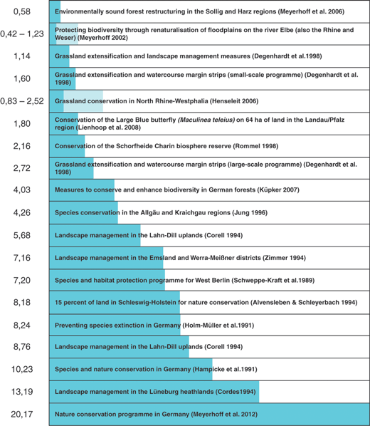
Fig. 4.9
Willingness-to-pay for conservation programmes encompassing various spatial and substantive factors (in €/mo.). When comparing the data, one matter to consider is that no adjustment was made for inflation. (Adapted and supplemented from BfN 2012 (references other than Meyerhoff et al. 2012 see there))
Some authors argue that concrete locally visible measures should be queried as much as possible, this provides a more realistic assessment of willingness-to-pay (Fischer and Menzel 2005). On the other hand, results regarding smaller, more specific measures always leave the question unanswered as to how the group of those questions regarding willingness-to-pay is to be defined: only at the municipality level, or that of the district, of the entire state, or nationwide? When questioned at the local level, one has to deal with the effect that measures in sparsely populated areas tend to always obtain a lower value than measures in densely populated areas, because of the smaller population, and hence the smaller potential willingness-to-pay group. For the valuation of nature as an ‘intrinsic value,’ this would be a substantively unacceptable result. Moreover, it has been demonstrated that the evaluation of specific measures always includes the implicit distributional assumptions of the respondents (‘If I pay for Measure A, I assume that others will pay for Measure B’; Degenhardt and Gronemann 1998). As an evaluation of ◉ Fig. 4.9 shows, a lower willingness-to-pay does tend to be expressed for special measures than for comprehensive measures; however, at the local and regional levels, the willingness-to-pay per measures unit is considerably higher. In the case of the preservation of the dusky large blue butterfly (Glaucopsyche nausithous) in Landau, the conversion of the willingness-to-pay results of the population to a per-ha of measure-implementation value yields € 6656/ha/yr. However, in a nationwide programme examined by Meyerhoff et al. (2012), values of only € 1000/ha for the specific grassland-part of the programme, exclusively, were obtained and 300 €/ha if the whole programme was valued. Actual per ha costs of conservation measures are usually below these figures.
For concrete decisions on conservation projects or interventions at the state or federal levels, the effect due to different population densities, regional preferences or implicit distributional assumptions are not particularly helpful. Such decisions should therefore be based on willingness-to-pay analyses, with which comprehensive programmes have been evaluated. Special willingness-to-pay for individual measures within these programmes could then be roughly evaluated on a pro rata basis, for instance per area segment, or, more accurately, through more detailed expert-based scoring methods (Schweppe-Kraft 1998).
Restoration-Cost Method
A nonpreference-based method for the assessment of existence values is the restoration-cost method. It is especially applied for the evaluation of the functions or services of habitats for the preservation of biodiversity. Under this method, the costs which would accrue if one were to first destroy a habitat and then restore it, are ascertained.
If restoration is required by law, this method is only used to ascertain what a measure, such as the construction of a road, would additionally cost in the form of mandatory compensatory measures. If restoration is not required, it ascertains the costs which would be incurred if society were to recognise in the future that restoration were necessary or desirable. Under economic theory, this approach is acceptable, since international conventions and policy statements such as the European Biodiversity Strategy have made a commitment to a ‘no-net-loss’ strategy with respect to the conservation of biological diversity. This means that we can–hopefully–assume with a relatively high degree of probability that such a restoration will in fact occur in the future.
A particular challenge in restoration-cost methodology is the monetisation of interim losses of function. Unlike technical infrastructure, the restoration of the biodiversity of ecosystems is not completed with the conclusion of the restoration of physical initial conditions (e.g. termination of intensive use, rewetting), but rather well, beyond that, require a number of years or even centuries. A number of different methods exist for evaluating the interim loss of function (Schweppe-Kraft 1998; Dietrich et al. 2014). In the USA, a discounting procedure within the framework of the so-called habitat equivalency analysis has been widely used since about 1995 for the quantification of damages. Previously, this method had already also been proposed for use in Germany for the assessment of tree damage and damage to habitats (Buchwald 1988; Schweppe-Kraft 1996; ▶ Sect. 6.6.1). The restoration-cost approach is also used in the German impact-regulation system (Köppel et al. 2004).
If this method is used to assess the approximately 10 % of Germany, which are of particular significance for the conservation of biological diversity, we obtain values of between 50 cents/m2 for farmland with endangered segetal plants and almost € 200/m2 for intact raised bogs. The total value of this 10 % of the land area in Germany comes to approximately € 740 billion, which, at the time of calculation, equaled some 80 % of the value of German productive capital (◉ Table 4.1).
Table 4.1
Compensation values for habitats in Germany, calculated analogously to the Habitat Equivalancy Analysis method, taking into account average recovery costs and times (Schweppe-Kraft 2009)