Loans and Risk Management Considerations

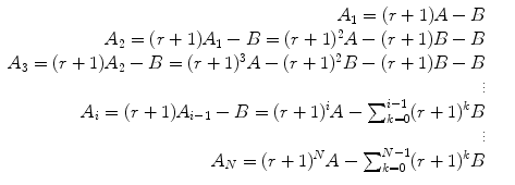
, the following relationship is derived:

(2.1)
This implies that the installment is equal to the difference in outstanding capital between two consecutive years (A t , A t+1) and the interest payment rA t . Equation (2.1) can be rewritten as  , where
  . This means that:

But A N = 0, therefore:

 , where
  . This means that:
(2.2)

(2.3)
Spreadsheets can easily handle such calculations, enabling users to build powerful models and plans. Equation (2.3) suggests that the higher the interest, the higher the installment B and the longer the duration N of the loan, the closer B is to the interest payment—i.e. B = A r , when. Furthermore, one can quickly calculate the expected payments, given A, r and N. Thus, in the numerical example where A = US$25 m, r = 7 % and N → ∞ years, the instalment B = US$4,186,694 is derived. Tables 2.1 and 2.2 indicate the sensitivity of the instalment over various years of duration and interest rates as well as the extent of difference from the given original case.
Table 2.1
Instalment: interest vs. duration of the loan
4 % | 5 % | 6 % | 7 % | 8 % | 9 % | 10 % | |
|---|---|---|---|---|---|---|---|
4 | 6,887,251 | 7,050,296 | 7,214,787 | 7,380,703 | 7,548,020 | 7,716,717 | 7,886,770 |
5 | 5,615,678 | 5,774,370 | 5,934,910 | 6,097,267 | 6,261,411 | 6,427,311 | 6,594,937 |
6 | 4,769,048 | 4,925,437 | 5,084,066 | 5,244,895 | 5,407,885 | 5,572,995 | 5,740,185 |
7 | 4,165,240 | 4,320,495 | 4,478,375 | 4,638,830 | 4,801,810 | 4,967,263 | 5,135,137 |
8 | 3,713,196 | 3,868,045 | 4,025,899 | 4,186,694 | 4,350,369 | 4,516,859 | 4,686,100 |
9 | 3,362,325 | 3,517,252 | 3,675,556 | 3,837,162 | 4,001,993 | 4,169,970 | 4,341,013 |
10 | 3,082,274 | 3,237,614 | 3,396,699 | 3,559,438 | 3,725,737 | 3,895,502 | 4,068,635 |
Table 2.2
Difference from the original instalment: interest vs. duration of the loan
4 % | 5 % | 6 % | 7 % | 8 % | 9 % | 10 % | |
|---|---|---|---|---|---|---|---|
4 | 64.5 % | 68.4 % | 72.3 % | 76.3 % | 80.3 % | 84.3 % | 88.4 % |
5 | 34.1 % | 37.9 % | 41.8 % | 45.6 % | 49.6 % | 53.5 % | 57.5 % |
6 | 13.9 % | 17.6 % | 21.4 % | 25.3 % | 29.2 % | 33.1 % | 37.1 % |
7 | −0.5 % | 3.2 % | 7.0 % | 10.8 % | 14.7 % | 18.6 % | 22.7 % |
8 | −11.3 % | −7.6 % | −3.8 % | 0.0 % | 3.9 % | 7.9 % | 11.9 % |
9 | −19.7 % | −16.0 % | −12.2 % | −8.3 % | −4.4 % | −0.4 % | 3.7 % |
10 | −26.4 % | −22.7 % | −18.9 % | −15.0 % | −11.0 % | −7.0 % | −2.8 % |
Borrowers and lenders often agree on terms such as interest payment on the outstanding capital, negotiate a balloon or a bullet loan,2 or decide on a grace period where no capital repayment is expected. Based on the following example, the differences in financing costs are clearly exposed in Tables 2.3 (outstanding capital), 2.4 (repayment with a grace period of 2 years) and 2.5 (bullet payment). In all these tables, the difference Diff. indicates the difference from the fixed interest payment of the first case. Table 2.6 summarises the cost of financing, i.e. the cumulative interest payment; it is clear that the bullet payment and the grace period schedule are the most expensive to borrowers. The substantially lower interest payments at the beginning of the loan period are compensated with substantially higher payments at the end. This could also raise concerns regarding the repayment capabilities of the borrowers; therefore, lenders might opt for a more conservative approach to the payment schedule. A counterargument that supports lower CapEx through a grace period scheme or a similar one at the early stages of the project suggests the reduced financial burden at the beginning, when liquidity is often at stake.
Table 2.3
Interest payment on the outstanding capital
Outstanding capital | Interest | Capital | Installment | Diff. | |
|---|---|---|---|---|---|
1 | 25,000,000 | 1,750,000 | 3,125,000 | 4,875,000 | 16.4 % |
2 | 21,875,000 | 1,531,250 | 3,125,000 | 4,656,250 | 11.2 % |
3 | 18,750,000 | 1,312,500 | 3,125,000 | 4,437,500 | 6.0 % |
4 | 15,625,000 | 1,093,750 | 3,125,000 | 4,218,750 | 0.8 % |
5 | 12,500,000 | 875,000 | 3,125,000 | 4,000,000 | − 4. 5 % |
6 | 9,375,000 | 656,250 | 3,125,000 | 3,781,250 | − 9. 7 % |
7 | 6,250,000 | 437,500 | 3,125,000 | 3,562,500 | − 14. 9 % |
8 | 3,125,000 | 218,750 | 3,125,000 | 3,343,750 | − 20. 1 % |
Table 2.4
Interest payment on the outstanding capital (grace period of 2 years granted)
Outstanding capital | Interest | Capital | Instalment | Diff. | |
|---|---|---|---|---|---|
1 | 25,000,000 | 1,750,000 | 0 | 1,750,000 | − 58. 2 % |
2 | 25,000,000 | 1,750,000 | 0 | 1,750,000 | − 58. 2 % |
3 | 25,000,000 | 1,750,000 | 4,166,667 | 5,916,667 | 41.3 % |
4 | 20,833,333 | 1,458,333 | 4,166,667 | 5,625,000 | 34.4 % |
5 | 16,666,667 | 1,166,667 | 4,166,667 | 5,333,333 | 27.4 % |
6 | 12,500,000 | 875,000 | 4,166,667 | 5,041,667 | 20.4 % |
7 | 8,333,333 | 583,333 | 4,166,667 | 4,750,000 | 13.5 % |
8 | 4,166,667 | 291,667 | 4,166,667 | 4,458,333 | 6.5 % |
Table 2.5
Bullet payment
Outstanding capital | Interest | Capital | Instalment | Diff. | |
|---|---|---|---|---|---|
1 | 25,000,000 | 1,750,000 | 0 | 1,750,000 | − 58. 2 % |
2 | 25,000,000 | 1,750,000 | 0 | 1,750,000 | − 58. 2 % |
3 | 25,000,000 | 1,750,000 | 0 | 1,750,000 | − 58. 2 % |
4 | 25,000,000 | 1,750,000 | 0 | 1,750,000 | − 58. 2 % |
5 | 25,000,000 | 1,750,000 | 0 | 1,750,000 | − 58. 2 % |
6 | 25,000,000 | 1,750,000 | 0 | 1,750,000 | − 58. 2 % |
7 | 25,000,000 | 1,750,000 | 0 | 1,750,000 | − 58. 2 % |
8 | 25,000,000 | 1,750,000 | 25,000,000 | 26,750,000 | 538.9 % |
Table 2.6
Comparison of the cost of financing
Method | Interest | Diff. |
|---|---|---|
Fixed | 8,493,552 | 7.9 % |
On the outstanding | 7,875,000 | 0.0 % |
Grace of 2 years | 9,625,000 | 22.2 % |
Bullet | 14,000,000 | 77.8 % |
The loan calculations are similar to many amortisation financial schemes and provide the basis for the estimation of capital expenses (CapEx).
2.1.2 Financial Viability Criteria
2.1.2.1 The NPV and IRR Criteria
Given the schedule of the loan, it is possible to proceed to more complicated calculations related to the project. In shipping projects, the NPV, RFR, and IRR criteria are considered more frequently. The NPV and the IRR are directly interrelated, while the NPV and the RFR are also conceptually intertwined.
The NPV calculations result in a discounted stream of annual profits or losses using the following formula:

where r is the discount rate—in most cases, this discount rate equals the opportunity cost of capital or reveals the expected rate of return on an investment in financial markets with similar risk—and N is the duration of the project. Given the maritime business environment, the revenues are commonly proceeds from a time charter (T/C), contract of affreightment or income from employment, e.g. from the spot market. On the other hand, capital (CapEx) and operating (OpEx) expenses as well as expenses related to voyages (VoyEx) should be taken into account, given the employment and operational pattern. If the outcome of the NPV calculation is positive, then this is a potentially lucrative project that should be financed. On the basis of formula (2.4), the IRR is estimated when NPV0 and the discount rate r is approximated numerically. Microsoft Excel T M supports functions for all these calculations. NPV is not a widely accepted criterion in shipping, as it is sensitive to the discount rate r, and the IRR criterion is potentially risky, as the formula might have multiple roots within a given space. Thus, both NPV and IRR criteria should be used cautiously. The IRR criterion neglects the size and risk characteristics of the investment, while the NPV is sensitive to the discount rate r, which, sometimes, is either fluctuating or not necessarily known.

(2.4)
2.1.2.2 Required Freight Rate
The RFR criterion is a variation of the NPV formula and is calculated based on a given ship (asset). This criterion determines the economic feasibility of a project at its early design stages, indicating the minimum required freight that sets NPV = 0, thereby indicating the point of indifference of the investor. Expected freight rates higher than the RFR deem the project profitable. Given formula 2.4, the RFR formula is expressed as:

where:

(2.5)